Introduction to SpreadsheetML

Since the introduction of Microsoft® Office XP, it is possible to create spreadsheets using SpreadsheetML, an XML dialect developed by Microsoft to represent the information in an Excel spreadsheet. This kind of document is referred to as an XML spreadsheet. Because XML spreadsheets are text documents, they can be sent wherever a text document can, using any text-based messaging system (for example, e-mail, Web services, and Web-based applications). In addition, an XML spreadsheet can be processed by any XML processor, making XML spreadsheets true cross-platform documents. An XML spreadsheet can be created with any text-editing tool.

This document covers most of the SpreadsheetML dialect. The document begins with a quick tour through the simplest possible XML spreadsheet, touching on each of the components necessary to build a functioning spreadsheet. In subsequent sections, these components are defined in more detail. You also see how to work with other features of Excel workbooks, such as PivotTables and XML document mapping. Almost everything in the SpreadsheetML dialect is an add-on to the base XML spreadsheet, so you can incorporate into an XML spreadsheet only those features that you want.

Keep in mind that the order in which the elements are discussed here is not necessarily the order that the elements must have in a spreadsheet for that spreadsheet to be a valid XML document.

Getting Started: The Simplest XML Spreadsheet

A single XML spreadsheet can, in fact, contain multiple spreadsheets. In Microsoft® Office Excel, the file that is created when you save your work is referred to as a workbook, which can contain one or more worksheets. This terminology is reflected in SpreadsheetML. The root element for an XML spreadsheet is the Workbook element. A Workbook element, in turn, can contain multiple Worksheet elements.

The simplest possible workbook that can be opened by Excel looks like this:

<?xml version="1.0"?>
<?mso-application progid="Excel.Sheet"?>
<Workbook
    xmlns="urn:schemas-microsoft-com:office:spreadsheet"
    xmlns:ss="urn:schemas-microsoft-com:office:spreadsheet">
<Worksheet ss:Name="Sheet1">
</Worksheet>
</Workbook>

XML Spreadsheets and Excel

The XML declaration in the first line of the foregoing example is normally optional in an XML document. If you omit it, however, Excel does not display the spreadsheets in the workbook correctly (see Figure 1).

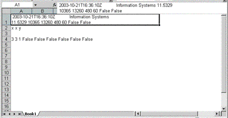
Figure 1. An Excel workbook without the XML declaration

The mso-application processing instruction in the example directs Microsoft Windows® to open the file in Excel when the user double clicks it, even if the file is saved with the .xml file name extension (for example, "MySpreadsheet.xml"). You can also save the file with the standard Excel file name extension (.xls). If you save an XML file with the .xls file name extension, you can omit the mso-application processing instruction, if you want, because in Windows the file is associated with Excel based on the file name extension.

When you save a document, Excel retains the format the document had when it is saved, regardless of the file name extension.

The Workbook element is the root element for the XML spreadsheet. Each Worksheet element within the Workbook element defines a worksheet that is displayed in Excel.

Excel Namespaces

In order to understand the format of an XML spreadsheet, you must understand the namespaces used by the XML spreadsheet. To begin with, the SpreadsheetML elements that make up the Excel XML dialect are divided into three groups of elements:

• Base spreadsheet functionality
• New functionality in Microsoft Office Excel 2003 (primarily, mapping XML documents)

Everything else in Microsoft Excel 2002, including data analysis tools (for example, PivotTable® views)

In addition, Excel spreadsheets can include HTML tags, SOAP tags, and tags from other XML dialects. To keep tags from different dialects separate, namespaces are used in XML.

A namespace is an arbitrary string of characters that is associated with a set of tags. Excel can distinguish among tags with the same name in XML spreadsheets because these tags are qualified by specific namespaces. Namespace qualification allows the Excel XML designers to use, for example, an Excel XML element called Table that does not conflict with the <table> tag in HTML. The SpreadsheetML Table element is associated with one of the Excel namespaces, and the HTML <table> tag is associated with the HTML namespace. Applications like Excel, therefore, that are designed to process XML documents can distinguish the two tags from each other, and process them according to different rules.

In the following sample, two namespaces are defined for the Workbook element (one is defined twice):

<Workbook
  xmlns:x="urn:schemas-microsoft-com:office:excel"
  xmlns="urn:schemas-microsoft-com:office:spreadsheet"
  xmlns:ss="urn:schemas-microsoft-com:office:spreadsheet">

The last two lines include ":spreadsheet" in the namespace definition. This is the SpreadsheetML namespace that qualifies tags associated with defining spreadsheet functionality. (This namespace is referred to as the spreadsheet namespace in this document.) The last line associates the spreadsheet namespace with the prefix "ss:". Any element with the "ss" prefix is associated with the spreadsheet namespace. In the previous line, the spreadsheet namespace is not associated with any particular prefix. Because the second line doesn't include a prefix, the spreadsheet namespace is the default namespace for the Workbook element and any of its child elements. In other words, any tag in the document that has no prefix is associated by default with the spreadsheet namespace.

For example, in the following sample, the Name attribute includes the "ss" prefix, so the Name attribute is considered part of the spreadsheet namespace. The Workbook and Worksheet elements, on the other hand, don't include the prefix, but they are nevertheless associated with the spreadsheet namespace because that namespace is defined for xmlns here without a prefix qualification:

<Workbook
  xmlns:x="urn:schemas-microsoft-com:office:excel"
  xmlns="urn:schemas-microsoft-com:office:spreadsheet"
  xmlns:ss="urn:schemas-microsoft-com:office:spreadsheet">
<Worksheet ss:Name="Sheet1">
</Worksheet>
</Workbook>

The following example uses the ExcelWorkbook element. In this example, the elements used to control the size and position of the window for the workbook in Excel have been included:

<?xml version="1.0"?>
<?mso-application progid="Excel.Sheet"?>
<Workbook 
  xmlns:x="urn:schemas-microsoft-com:office:excel"
  xmlns="urn:schemas-microsoft-com:office:spreadsheet"
  xmlns:ss="urn:schemas-microsoft-com:office:spreadsheet">

    <x:ExcelWorkbook >
        <x:WindowHeight>9120</x:WindowHeight>
        <x:WindowWidth>10005</x:WindowWidth>
        <x:WindowTopX>120</x:WindowTopX>
        <x:WindowTopY>135</x:WindowTopY>
    </x:ExcelWorkbook>
</Workbook>

The ExcelWorkbook element and its child elements have the "x" prefix. This prefix associates these elements with the namespace that ends with ":excel", which is defined in the Workbook element along with the spreadsheet namespace. (This namespace is referred to as the "Excel namespace" in this document.)

Getting the right elements into the right namespaces is critical to creating a valid Excel XML spreadsheet. Excel does not properly process a SpreadsheetML tag unless it is tied to the correct namespace.

An XML spreadsheet created in Excel, however, does not always associate elements with namespaces by using prefixes. For example, Excel generates the ExcelWorkbook element like this:

<ExcelWorkbook xmlns="urn:schemas-microsoft-com:office:excel">
    <WindowHeight>9120</WindowHeight>
    <WindowWidth>10005</WindowWidth>
    <WindowTopX>120</WindowTopX>
    <WindowTopY>135</WindowTopY>
</ExcelWorkbook>

In this example, the Excel namespace is declared in the ExcelWorkbook element. Because no prefix is used, the Excel namespace is the default namespace for the ExcelWorkbook and its child elements. As a result, no prefixes are required for these elements to associate them with the Excel namespace.

When you create XML spreadsheets, you can use whichever technique you prefer to associate elements with namespaces. You can declare namespaces globally and use prefixes throughout the document, or you can declare namespaces locally and avoid the use of prefixes. As long as elements are associated with suitable namespaces, Excel processes the document correctly.

In order to be clear about which elements belong to which namespaces, all elements and attributes in the examples in this article is given a prefix to identify the namespaces to which they belong. You should read the examples as if namespaces have been declared globally and no default prefix is defined. The prefixes used are the same as those that Excel uses when it creates an XML spreadsheet. The prefixes used most often are the following:

• ss: the spreadsheet namespace ("urn:schemas-microsoft-com:office:spreadsheet")
• x: the Excel namespace ("urn:schemas-microsoft-com:office:excel")
• x2: the Excel2 namespace ("urn:schemas-microsoft-com:office:excel2")

Keep in mind that the examples in this article won't look exactly like XML spreadsheets generated by Excel. In XML spreadsheets generated by Excel, namespace prefixes are not used nearly as often as locally defined namespaces.

Referencing cells

In formulas that reference cells in XML spreadsheets, the R1C1 reference style is used instead of the A1 reference style. Using R1C1 notation, cell B2, for example, is referenced as "R2C2" (row 2, column 2). In the following sample, a formula is defined in a cell's Formula attribute that adds the values from cells A1 and A2:

<ss:Cell ss:Formula="=R1C1+R2C1">

Cell references in the R1C1 style can be created with absolute or relative addresses. From the point of view of the developer creating an XML spreadsheet, absolute addresses are easier to create. For example, the formula "=R1C1+R2C2" uses absolute addresses. (In the formula bar in Excel, this formula would appear as "=$A$1+$B$2".) Relative addresses are more difficult to write and to read. On the other hand, if (in Excel) the user copies a cell with a formula that uses absolute addresses to a new location, that formula still refers to the same cells as it did in its original location. This behavior may not be what the user expects.

Suppose, for example, that cell B5 contains the formula "=R3C2+R4C2" (In A1 reference style: "=B3+B4"). If, in Excel, the user copies the contents of this cell to cell C5, the formula in C5 remains unchanged— the value displayed is still the result of adding cells B3 and B4.

If the user copies a cell with a formula that uses relative addresses to a new location, the formula addresses a different set of cells, based on its new position. To use relative addresses, the cell references must be offsets from the cell containing the formula. A formula in cell B5 that added cells B3 and B4 would be expressed using relative addresses as "=R[-2]C+R[-1]C". If, in Excel, the user copies this formula to cell C5, the formula would add cells C3 and C4. In relative addressing, zeroes are omitted, so "RC[-2]" refers to the cell two columns to the left in the same row. (In relative addressing, the current cell is identified as "RC".

The Structure of an XML Spreadsheet

In this section, you'll be introduced to the overall structure of the Workbook element beginning with the child elements of the Workbook element itself and continuing down to the individual cells in the spreadsheet. The Workbook element contains numerous child elements in addition to the Worksheet element. (The Workbook element has no attributes.) The following table lists the child elements of the Workbook element, in the order in which they must be specified. Most of these elements are optional.

Table 1. Elements of the Workbook element

Constructing a Spreadsheet

The heart of an XML spreadsheet is the spreadsheet itself. The elements that make up a spreadsheet is therefore discussed first. Subsequent sections of this article cover the Worksheet element, which contains the spreadsheet and the other child elements of the Workbook element.

All of the elements discussed in this section are members of the spreadsheet namespace. These tags constitute most of the functionality of the data calculation engine in Excel. These elements were designed to simplify "hand-coding"— it should be possible to create a functioning spreadsheet using any text editor. Other functionality, primarily from the Excel namespace, is more complicated to implement in an XML spreadsheet. A PivotTable, for example, requires numerous interrelated tags.

The Table Element: A Container for the Spreadsheet

Within a Worksheet element, a hierarchy of elements defines a spreadsheet:

• Table: Holds the row elements that define a spreadsheet
• Row: Holds the cell elements that make up a row
• Cell: Holds the data for an individual cell

In addition, Column elements (children of the Table element) can be used to define the attributes of columns in the spreadsheet.

The following example puts numbers in cells A1 and B2, and a formula that adds these numbers in cell D5. The Index attribute specifies the row and cell numbers, but it can be omitted if the cell or the row is the first cell or row in the spreadsheet, or the Cell or Row element represents the next cell or row in the spreadsheet. (The spreadsheet can be seen in Figure 2.)

<ss:Table>
   <ss:Row>
       <ss:Cell>
           <ss:Data ss:Type="Number">1</ss:Data>
       </ss:Cell>
   </ss:Row>
   <ss:Row>
       < ss:Cell ss:Index="2">
           < ss:Data ss:Type="Number">3</ss:Data>
       </ss:Cell>
   </ss:Row>
   <ss:Row ss:Index="5">
       <ss:Cell ss:Index="4" ss:Formula="=R1C1+R2C2">
           <ss:Data ss:Type="Number">4</ss:Data>
       </ss:Cell>
   </ss:Row>
</ss:Table>

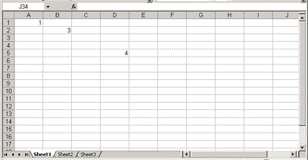
Figure 2. An Excel workbook window displayed in Excel

As the example shows, formulas are contained in the Formula attribute of a Cell element and the contents of the cell are in the Data element, which is a child of the Cell element. Because an XML spreadsheet is an XML document, any reserved XML characters in strings must be replaced with their corresponding entities or the entire string must be enclosed in a CDATA section (see Appendix 7 for a list of reserved XML characters). For example, the text "Hello, World" (including the double quotes) would need to be written either like this:

<ss:Data ss:Type="String">&quot;Hello, world&quot;</ss:Data>

or like this:

<ss:Data ss:Type="String"><![CDATA["Hello, world"]]></ss:Data>

Defining Rows

Only cells that contain data need to be defined in the XML spreadsheet. In the previous example, there is data in rows 1, 2, and 5 only, so there are only three Row elements in the document. Further, as long as the rows are consecutive, you don't have to specify the row number in the Index attribute of the Row element.

These XML elements would define the first two rows in a spreadsheet:

<ss:Table>
   <ss:Row>
   ...row information...
   </ss:Row>
   <ss:Row>
   ...row information...
   </ss:Row>

In the following example, however, rows 1, 3, and 5 contain no data, so the Row elements for the existing rows use the Index attribute to specify what rows they are defining:

<ss:Table>
   <ss:Row ss:index="2">
   ...row information...
   </ss:Row>
   <ss:Row ss:index="4">
   ...row information...
   </ss:Row>
   <ss:Row ss:index="6">
   ...row information...
   </ss:Row>

Once a row in a series of rows contains a specification for its position, it is not necessary for subsequent rows to include an Index attribute, as long as no rows are omitted. The following example defines rows 4 and 5. Although row 4 needs an index, row 5 does not:

<ss:Table>
   <ss:Row ss:index="4">
   ...row information...
   </ss:Row>
   <ss:Row>
   ...row information...
   </ss:Row>

You can include Index attributes in all Row elements without generating errors, but, as seen in the foregoing examples, indexes are not always necessary.

Defining Cells

Within a Row element, the Cell element defines the row's cells in a way very similar to the way that rows are defined: only the cells that contain data appear in the document. As with the Row element, the Index attribute of the Cell element specifies the column in which that cell appears. Also, as it is for a row, only the first cell following an empty column in the same row requires an Index attribute. The following example defines the cells for columns 1, 2, 4, 5, and 7. Note where Index attributes are explicit:

<ss:Row>
   <ss:Cell></ss:Cell>
   <ss:Cell></ss:Cell>
   <ss:Cell ss:Index="4"></ss:Cell>
   <ss:Cell></ss:Cell>
   <ss:Cell ss:Index="7"></ss:Cell>
</ss:Row>

Adding data and formulas to cells is discussed in the section "Putting Data in the Cell."

Defining Columns

The row-and-cell model of SpreadsheetML doesn't directly support the concept of a spreadsheet column. In order to control the columns of a spreadsheet as a unit (rather than as a collection of cells), you can use the Column element. All Column elements for a spreadsheet must follow the Table element and precede the first Row element.

The Column element has five attributes:

• Width: The width of the column (in points)
• Hidden: When set to 1, the column is not displayed in Excel
• AutoFitWidth: When set to 1, the column is automatically sized in Excel to display the entire length of numeric and date values. When set to 0, no autosizing takes place. (Columns are not automatically re-sized for other data types.)
• Span: Eliminates the need to include Column elements for a set of columns with the same values specified in their attributes.

AutoFitWidth and Width affect each other as described in Table 2.

Table 2. The relationship between the AutoFitWidth and Width attributes

Setting the Span attribute of a Column element to 5 causes the five columns to the right of the Column element with the Span attribute to be formatted exactly like that Column element. In the following example, the three columns to the right of column 2 in the spreadsheet (that is, columns 3, 4, and 5) have the same formatting as column 2:

<ss:Table>
    <ss:Column ss:Index="2" ss:Width="500" ss:Span="3"/>
</ss:Table>

If the subsequent Column element does not have an Index attribute, then that Column element defines the first column to follow the span. In the next example, the second Column element defines column 6:

<ss:Table>
    <ss:Column ss:Index="2" ss:Width="500" ss:Span="3"/>
    <ss:Column ss:Width="200" />
</ss:Table>

Attempting to define a column twice, either by specifying the same index for two Column elements or by specifying an index explicitly that has already been used implicitly for a column in a span of columns generates an error in Excel. All the following examples would generate errors in Excel because they define column 2 more than once:

<ss:Table>
    <ss:Column ss:Width="200" ss:Span="1"/>
    <ss:Column ss:Index="2" ss:Width="200" />
</ss:Table>

<ss:Table>
    <ss:Column ss:Index="2" ss:Width="500" />
    <ss:Column ss:Index="2" ss:Width="250" />
</ss:Table>
<ss:Table>
    <ss:Column ss:Width="1000" />
    <ss:Column ss:Width="500" />
    <ss:Column ss:Index="2" ss:Width="250" />
</ss:Table>

Shifting the Table

If multiple Table elements are found in a Worksheet element, Excel processes only the first Table element (without generating an error). When the spreadsheet is saved, Excel discards all but the first table.

This design allows Excel in the future to support multiple overlapping ranges by having multiple Table elements. To support this, the Table element has a LeftCell and a TopCell attribute. These attributes control the position of the Table within the worksheet. If these attributes are not specified, they default to 1.

Within a Table element, many references are based on the values in the LeftCell and TopCell attributes. The Index attributes in the Row and Cell elements, For example, are calculated based on the values of the TopCell and LeftCell attributes. As an example, setting the LeftCell and TopCell attributes to 20 would cause all rows and cells to be moved 20 columns to the right and 20 columns down. Relative addresses in formulas are not disrupted by setting the TopCell and LeftCell values because relative addresses in a formula are always based on the cell containing the formula. Absolute addresses, however, are affected by changes to the values of the TopCell and LeftCell attributes.

It is important to note that Excel does not retain the values of the TopCell and LeftCell attributes when an XML spreadsheet is saved. These values are discarded and Index attributes are set based on the default values of the TopCell and LeftCell attributes (that is, a value of 1).

Cells

Cell Contents

The contents of a cell can be divided into two categories: formulas and data. Formulas are discussed later. This section explains how to put data into a cell.

Cell Data

Within the Cell element, the Data element contains the value of a cell. If the cell contains a formula that calculates a value dynamically, the Data element contains the current value resulting from the formula. The Data element has a Type attribute, which specifies the data type of the data in the cell. Valid values for the Type attribute are Number, DateTime, Boolean, String, and Error. The following example specifies a cell that contains a string:

<ss:Cell>
   <ss:Data ss:Type="String">Monday</ss:Data>
</ss:Cell>

Cell Comments

In addition to a Data element, a Cell element may contain a Comment element, which contains a comment for the cell. The Comment element has two attributes:

• Author: The name of the comment's author
• ShowAlways: A value of 1 for this attribute indicates that the comment is always to be displayed

The text that makes up the comment is kept in a Data element within the Comment element, and that text can be formatted with HTML tags. In the following example, a cell has a comment containing the string "Author: The first day of the week":

<?xml version="1.0"?>
<?mso-application progid="Excel.Sheet"?>
<Workbook xmlns="urn:schemas-microsoft-com:office:spreadsheet"
   xmlns:x="urn:schemas-microsoft-com:office:excel"
   xmlns:ss="urn:schemas-microsoft-com:office:spreadsheet"
   xmlns:html="http://www.w3.org/TR/REC-html40">
    <Worksheet ss:Name="Sheet1">
        <ss:Table>
            <ss:Row>
                <ss:Cell>
                    <ss:Data ss:Type="String">Monday</ss:Data>
                    <ss:Comment ss:Author="Author" ss:ShowAlways="1">
                        <ss:Data><html:B><html:Font html:Face="Tahoma" html:Size="8" html:Color="000000">Author:</html:Font></html:B>
                        <html:Font html:Face="Tahoma" html:Size="8" html:Color="000000">&10;The </html:Font><html:B>
                        <html:Font html:Face="Tahoma" x:Family="Swiss" html:Size="8" html:Color="000000">first</html:Font></html:B>
                        <html:Font html:Face="Tahoma" x:Family="Swiss" html:Size="8" html:Color="000000"> day of the week.</html:Font>
                        </ss:Data>
                    </ss:Comment>
                </ss:Cell>
            </ss:Row>
        </ss:Table>
    </Worksheet>
</Workbook>

In this example, all of the HTML elements and attributes have been given the prefix "html" to associate these elements and attributes with to the HTML namespace. The HTML namespace be declared in some ancestor element (for example, the root element of the document), using the html prefix:

xmlns:html="http://www.w3.org/TR/REC-html40"

When Excel generates a spreadsheet that contains a comment, it declares the HTML namespace in two places:

• Globally, that is, in the Workbook element, using the prefix "html"
• Locally, that is, in the Data element within the comment, without a prefix

The Font element from the HTML namespace can also hold the Family attribute from the Excel namespace. This specifies the kind of font to use in the comment. In one of the Font elements in the foregoing example, For example, a Swiss font family is specified. (Other permissible values are: Decorative, Modern, Roman, and Script.) This information is used by Excel to select a substitute font if the font specified in the Face attribute of the Font element isn't available on the computer.

Cell Formulas

A key feature of Excel is the ability to store formulas in cells. In an XML spreadsheet, the Formula attribute of a Cell element contains the formula associated with the cell (if the cell has a formula). A formula consists of an equals sign (=) followed by calls to Excel functions, operators, values, and references to other cells (in R1C1 format).

Except for the R1C1 notation, formulas in an XML Spreadsheet follow the format used in the Excel formula bar. Ranges are expressed as two cell references separated by a colon. To reference the range C2 to C5, For example, you could use the absolute address R2C3:R5C3.

R1C1 cell references used in functions must be enclosed in parentheses. The next example uses relative cell references and, in cell C10, calculates the average of cells C2 to C9:

<ss:Cell ss:Index="3" ss:Formula="=AVERAGE(R[-8]C:R[-1]C)">

Because an XML spreadsheet is an XML document, any reserved characters in XML must be replaced by the appropriate entities (see appendix 7). The formula

= "X" &C19

must therefore be written like this:

="X" &R[5]C[1]

Of the five entities, the apostrophe doesn't always need to be replaced with its corresponding character entity, but it's a good practice to do so.

Cell names can be used in formulas without parentheses, as in this example, which refers to the cell called "MyName":

<ss:Cell ss:Formula="=MyName">

Array Formulas

In an array formula, only the cell in the top left corner of the array has a Formula attribute. This cell must also have an ArrayRange attribute that specifies the range for the result of the formula. The braces that appear in the Excel formula bar when you create an array formula are not required in an XML spreadsheet. The following example creates an array formula that multiplies the range B2:C2 by the range D2:E2, using absolute addresses. This formula returns a single result, so the ArrayRange attribute specifies current cell ("RC" in relative cell references):

<ss:Cell ss:ArrayRange="RC" 
ss:Formula="=SUM(R2C2:R2C3*R2C4:R2C5)">

References to Other Worksheets

Where the cell is in another worksheet in the same workbook, the name of the worksheet must precede the R1C1 reference and be separated from it with an exclamation mark. The following example references cell B2 in the sheet called MyOtherSheet:

<ss:Cell ss:Formula="=MyOtherSheet!R2C2">

If the name of the worksheet includes blanks or special characters, the name must be enclosed in single quotes:

<ss:Cell ss:Formula="='My Other Sheet'!R2C2">

References to Other Workbooks

When a cell involved in a formula is in a worksheet in a different workbook, you must include the name of the workbook and the relative or full path to the workbook in the formula. (If the workbooks are in the same folder, the path can be omitted). Enclose the file name of the workbook in square brackets. In addition, if the file name contains spaces or special characters, everything prior to the exclamation mark must be enclosed in single quotes.

The following example references the cell D4 in a worksheet called My Sheet, which itself is part of a workbook called MyOtherBook in a folder called OtherSheetsBecause the sheet name includes a space, everything between the equals sign and the cell reference is enclosed in single quotes:

<ss:Cell ss:Index="2" ss:Formula=
"='OtherSheets\[MyOtherBook.xls]My Sheet'!R4C4">
    <ss:Data  ss:Type="Number">321</ss:Data>
</ss:Cell>

Caching Data from Other Workbooks

The SupBook element holds data extracted from other workbooks. The SupBook element is a child of the ExcelWorkbook element and is a member of the Excel namespace. There is one SupBook element for every referenced workbook. The SupBook element maintains information about the spreadsheet being referenced. Excel extracts the data from the referenced workbooks and stores that data in the SupBook element, where it can be used in calculations without having to open the referenced workbook.

Excel creates SupBook elements if they aren't present, so it's not necessary to add SupBook elements explicitly to your XML spreadsheet. The SupBook element is described in detail in Appendix 4.

Other Cell Attributes

The Cell element can have three other attributes:

HRef: This attribute specifies a hyperlink. When a user clicks the cell, the link to the URL specified in the HRef attribute is activated. If you specify a URL in the Data element of a Cell element, the cell is not an active hyperlink— the contents of the cell are treated as a string of text. In the following example, a cell is defined with a hyperlink to the Microsoft Web site:

<ss:Cell ss:Index="7" ss:HRef="http://www.microsoft.com">
    <ss:Data ss:Type="String">Linked Cell</ss:Data>
</ss:Cell>

In the absence of any formatting in the XML spreadsheet, Excel displays the URL specified in the HRef attribute as plain text, that is, with none of the characteristics that users may associate with a hyperlink in other contexts (for example, in a Web browser). Formatting is discussed later in this document.

• MergeAcross, MergeDown: These two attributes contain the number of cells to be merged into the current cell when the spreadsheet is displayed in Excel.
• MergeAcross: Specifies the number of cells to the right of the current cell to be merged into the current cell. MergeDown specifies the number of cells below the current cell to be included in the merged with the current cell. This example causes the first cell in the row to be merged with the second cell:

<ss:Table>
    <ss:Row>
        <ss:Cell ss:MergeAcross="1"/>
    </ss:Row>
</ss:Table>

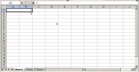
Figure 3. A spreadsheet with cells A1 and A2 merged

Merging cells changes the structure of the spreadsheet. For example, in the preceding previous example, cell 1 in the first row is merged with cell 2. The results can be seen in Figure 3. Cell 2 no longer exists in the first row. Any attempt to define a cell with an index of 2 for this row generates an error when the XML spreadsheet is processed by Excel. This XML example, for example, is not loaded by Excel because the second Cell element explicitly identifies itself as cell 2:

<ss:Table>
    <ss:Row>
       <ss:Cell ss:MergeAcross="1" />
       <ss:Cell ss:Index="2" />
    </ss:Row>
</ss:Table>

When the first two cells in the first row are merged, then, cell 2 in effect disappears from this row and cannot be used or referenced later. Because cell 2 has disappeared, the second Cell element in the following example represents the third cell in the row:

<ss:Table>
    <ss:Row>
        <ss:Cell ss:MergeAcross="1"/>
        <ss:Cell><ss:Data ss:Type="String">Third Cell</ss:Data>
        </ss:Cell>
    </ss:Row>
</ss:Table>

Managing the Worksheet

The Worksheet element has three attributes that allow you to control the worksheet. One of them, the Protected attribute, is described in the section on protection later in this document.

• Name: This attribute specifies the name for the Worksheet, and it is required. The value must conform to the rules for spreadsheet names in Excel, and it must not be the same as the name of any other worksheet in the workbook. In Excel, worksheets are displayed in the order that they appear in the XML document.
• RightToLeft: When set to 1, in versions of Excel that support displaying data from right to left, the spreadsheet is displayed with column A on the right-hand side instead of the left

In the following example, shown in Figure 4, the spreadsheet is given the name "XMLSample" and the value of the RightToLeft attribute is set to 1:

<ss:Worksheet ss:Name="Sheet1" ss:RightToLeft="1">

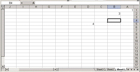
Figure 4. A sample worksheet displayed in right-to-left format

Defining Names

Defining names for cells is useful for creating maintainable spreadsheets, because you can replace obscure R1C1 cell references with meaningful names. Assigning a name to a cell or range in an XML spreadsheet requires you to coordinate two separate entries, one at the worksheet level and one at the cell level.

Defining a Named Range

The Names element of the Workbook element contains the elements that define the names used in the workbook. Within the Names element, a NamedRange element allows you to define a name for a range. The NamedRange element has the following three attributes:

• Name: This attribute specifies the name for the range. The value specified must follow the rules for names in Excel.
• Hidden: Setting the value of this attribute to 1 makes the range invisible in Excel.
• RefersTo: This attribute specifies the cell reference or range reference to which the Name attribute applies.

For named ranges, you must use absolute addressing in the RefersTo attribute. In addition, because names are defined at the workbook level, you must also include the name of the worksheet in which the range appears.

In the following example, a range called DefinedRange is defined, and it includes cells C1 to C4 in a worksheet whose Name attribute is set to "Sheet1":

<ss:Names>
    <ss:NamedRange ss:Name="DefinedRange" ss:RefersTo="=Sheet1!R1C3:R4C3"/>
</ss:Names>

It is not necessary for the cells in a named range to be contiguous. Multiple ranges can be included in the RefersTo attribute, with each range separated by a comma. The following example specifies two groups of cells to make up the named range:

<ss:Names>
    <ss:NamedRange ss:Name="DefinedRange" 
ss:RefersTo="=Sheet1!R1C3:R4C3, Sheet1!R3C3:R5C3"/>
</ss:Names>

To specify a name for a single cell, you define a NamedRange, referencing that individual cell only. In this example, the name "DefinedName" is assigned to cell C8:

<ss:Names>
    <ss:NamedRange ss:Name="DefinedName" 
ss:RefersTo="=Sheet1!R1C8"/>
</ss:Names>

After a cell is assigned a name, you can use that name in references to the cell. In the following example, a cell that is assigned a name is used in a formula associated with a different cell:

<Workbook
    xmlns="urn:schemas-microsoft-com:office:spreadsheet"
    xmlns:ss="urn:schemas-microsoft-com:office:spreadsheet"
<ss:Names>
    <ss:NamedRange ss:Name="DefinedRange" ss:RefersTo="=Sheet1!R1C3"/>
</ss:Names>
<Worksheet ss:Name="Sheet1">
    <ss:Table>
        <ss:Row>
           <ss:Cell />
           <ss:Cell><ss:Data ss:Type="String">Second Cell</ss:Data></ss:Cell>
           <ss:Cell><ss:Data ss:Type="Number">100</ss:Data></ss:Cell>
           <ss:Cell ss:Formula="=SUM(DefinedRange, 4)" />
        </ss:Row>
    </ss:Table>
</Worksheet>
</Workbook>

For a named range, in addition to the NamedRange element, each Cell element in the named range can have a NamedCell element with its Name attribute set to the name of the range. Cells that participate in multiple named ranges have multiple NamedCell elements. No error is raised if no cell has a matching NamedCell. If you omit the NamedCell element, Excel adds it when it saves the workbook.

Controlling the Spreadsheet Display

SpreadsheetML allows you to control how the spreadsheet as a whole is displayed in Excel. Formatting of individual cells is discussed later in this document.

Default Column Width and Row Height

Attributes of the Worksheet element allow you to specify, in points, the default column width and row height for the worksheet. In the following example, For example, the default column width is set to 20 points and the default row height is set to 30 points:

<ss:Worksheet ss:DefaultColumnWidth="20" ss:DefaultRowHeight="30">

If these attributes are not specified for the Worksheet element, the default column width is 48 points and the default row height is 12.75 points.

Positioning the Spreadsheet

You can also specify values for attributes of the Worksheet element that allow you to control how the spreadsheet is positioned in the worksheet window. The TopCell attribute specifies which row should be the top row in the window; the LeftCell attribute specifies which column should be the first column in the window. The values for both of these attributes must be an integers greater than 0. For example, to have the window display with the cell D5 in the upper left hand corner, you must set the 4^th column in the LeftCell attribute and the 5^th row in the TopCell attribute:

<ss:Worksheet  ss:LeftCell="4" ss:TopCell="5"
ss:DefaultColumnWidth="20" ss:DefaultRowHeight="30">

Figure 5 shows the results of these settings.

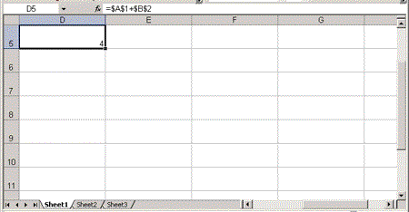
Figure 5. A worksheet configured with custom settings

You can also control which part of the spreadsheet is initially visible by using the TopRowVisible and LeftColumnVisible elements of the WorksheetOptions element. (These elements belong to the Excel namespace). These elements define the first row visible at the top of the screen (with row 1 at position 0) and the first column visible on the left edge (with column A at position 0). In the following example, the third row and the fourth column (column D) is the topmost and leftmost items, putting cell D3 in the upper left hand corner of the spreadsheet window:

<Worksheet ss:Name="Sheet1">
    <x:WorksheetOptions>
        <x:TopRowVisible>2</x:TopRowVisible>
        <x:LeftColumnVisible>3</x:LeftColumnVisible>
    </x:WorksheetOptions>
    <ss:Table>
        <ss:Row>
           <ss:Cell />
           <ss:Cell><ss:Data ss:Type="String">A cell</ss:Data></ss:Cell>
        </ss:Row>
    </ss:Table>

</Worksheet>

The ActiveSheet element controls which sheet is initially visible when a workbook is opened. For most of the sheets in a workbook, these settings only take effect when the user switches to the sheet. The ActiveSheet element specifies the sheet by its position in the workbook, with the first sheet at position 0. This example makes the second sheet in the workbook the active sheet:

<x:ExcelWorkbook>
<x:ActiveSheet>1</x:ActiveSheet>
</x:ExcelWorkbook>

You control the magnification level of the spreadsheet with the Zoom element in the WorksheetOptions element. The magnification level can range from 10% to 400% (see Figure 6 and 7). The following example sets the Zoom level to 250%:

<x:WorksheetOptions>
    <x:Zoom>250</x:Zoom>
</x:WorksheetOptions

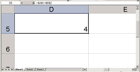
Figure 6. A spreadsheet at a zoom level of 400%

Figure 7. The same spreadsheet at a zoom level of 100%

Window Size and Position

Window height, width, and position are controlled by elements in the ExcelWorkbook element, which is a child of the Workbook root element. The WindowHeight and WindowWidth elements control the size of the window in which the workbook is displayed. These dimensions are specified in points. You control the position of the workbook window within the Excel window using the WindowTopX and WindowTopY elements. The WindowTopX sets the distance in points between the top of the workbook window to the top inside edge of the Excel window; the WindowTopY sets the distance between the left edge of the workbook window to the left inside edge of the Excel window. In the following example, the workbook window is set to 5000 points high and 5000 points wide, and the position of the window is set at 500 points from top of the workbook window and 250 points from the left edge:

<Workbook xmlns="urn:schemas-microsoft-com:office:spreadsheet"
   xmlns:x="urn:schemas-microsoft-com:office:excel"
   xmlns:ss="urn:schemas-microsoft-com:office:spreadsheet"
   xmlns:html="http://www.w3.org/TR/REC-html40">
<x:ExcelWorkbook>
    <x:WindowHeight>5000</x:WindowHeight>
    <x:WindowWidth>5000</x:WindowWidth>
    <x:WindowTopX>500</x:WindowTopX>
    <x:WindowTopY>250</x:WindowTopY>
</x:ExcelWorkbook>
<Worksheet ss:Name="Sheet1">
    <ss:Table>
        <ss:Row>
            <ss:Cell>
                <ss:Data ss:Type="String">A cell</ss:Data>
            </ss:Cell>
        </ss:Row>
    </ss:Table>
</Worksheet>
</Workbook>

The values of the WindowTopX and WindowTopY elements apply only when the workbook window isn't maximized. The values of the WindowHeight and WindowWidth elements do apply to a maximized workbook window, but the window is displayed with the dimensions specified in these elements only when the window is not maximized. (Whether or not the workbook window is maximized cannot be controlled by elements in the XML spreadsheet.)

Selected Sheets

You can also specify which sheets are selected in a workbook. (In Excel, a sheet is selected by clicking on its tab). To specify that a sheet is currently selected, add the Selected element to the WorksheetOptions element associated with that worksheet. In the following example, a worksheet named "Sheet3" is selected:

<x:Worksheet ss:Name="Sheet3">
    <x:WorksheetOptions>
        <x:Selected/>
    </x:WorksheetOptions>
</x:Worksheet

It is possible to have more than a single sheet selected. The Selected element must be added to the WorksheetOptions element of each selected sheet. In addition, the SelectedSheets element, which holds a count of the number of selected sheets, must be added to the ExcelWorkbook element. (If the SelectedSheets element isn't present, it defaults to 1, so the element isn't required when only a single sheet is selected.)

In the following example, both Sheet1 and Sheet3 are selected (but not Sheet2):

<x:ExcelWorkbook>
    <x:SelectedSheets>2</x:SelectedSheets>
<x:/ExcelWorkbook>
<x:Worksheet ss:Name="Sheet1">
    <x:WorksheetOptions>
        <x:Selected/>
    </x:WorksheetOptions>
</x:Worksheet
    <x:Worksheet ss:Name="Sheet2">
    <x:WorksheetOptions>
    </x:WorksheetOptions>
</x:Worksheet
<x:Worksheet ss:Name="Sheet3">
    <x:WorksheetOptions>
        <x:Selected/>
    </x:WorksheetOptions>
</x:Worksheet>

Selecting a sheet and making a sheet active are not the same thing. Only one sheet can be active at a time, but multiple sheets can be selected at the same time. The ActiveSheet element of the ExcelWorkbook element overrides the Selected element of the Worksheet element. That is, if you have specified the third spreadsheet of a workbook as the active sheet in the ExcelWorkbook element, then even if you add the Selected element to the second spreadsheet, the third spreadsheet is active— and selected— when you open the workbook.

Formatting: Styles and Conditional Formatting

In the Excel user interface, you can apply formatting to an individual cell or you can define a style and apply that style to one or more cells. In an Excel XML spreadsheet, only one formatting mechanism is available: you must define a style and then apply it to the cell.

Styles

A style is defined in the Styles element, which appears in an XML spreadsheet right after the ExcelWorkbook element and before the Worksheet element. Within the Styles element, individual Style elements define particular styles. The ID element of the Style element provides a unique identifier that can be used by other elements within the document. The Name attribute of a Style element provides a "friendly" identifier for the style.

The following sample illustrates a Styles element that contains the definition for two styles. The ID of the first Style element is "Default" and the value of the Name attribute is "Normal". The ID of the second Style element is "s22":

<Workbook xmlns="urn:schemas-microsoft-com:office:spreadsheet"
   xmlns:x="urn:schemas-microsoft-com:office:excel"
   xmlns:ss="urn:schemas-microsoft-com:office:spreadsheet"
   xmlns:html="http://www.w3.org/TR/REC-html40">
<x:ExcelWorkbook>
    <WindowHeight>10000</WindowHeight>
    <WindowWidth>10000</WindowWidth>
</x:ExcelWorkbook>
<ss:Styles>
    <ss:Style ss:ID="Default" ss:Name="Normal">
        <Font x:Family="Swiss" ss:Size="10" ss:Bold="0"/>
        <ss:Alignment ss:Vertical="Bottom"/>
    </ss:Style>
    <ss:Style ss:ID="s22">
        <Font x:Family="Swiss" ss:Size="12" ss:Bold="1"/>
        <ss:NumberFormat ss:Format="0.00;[Red]0.00"/>
    </ss:Style>
</ss:Styles>
<Worksheet ss:Name="Sheet1">
    <ss:Table>
        <ss:Row>
            <ss:Cell>
                <ss:Data ss:Type="String">Total</ss:Data>
            </ss:Cell>
            <ss:Cell ss:StyleID="s22">
                <ss:Data ss:Type="Number">-45</ss:Data>
            </ss:Cell>
        </ss:Row>
    </ss:Table>
</Worksheet>
</Workbook>

A style that has a Name attribute is displayed in the list of styles in the Style dialog box when the spreadsheet is opened in Excel. The first style in the foregoing example is called 'Normal' in the Excel Style dialog box, For example. The second style in the example doesn't have a name, so it won't appear in the Style dialog box.

The first style uses the Font element to specify a font style (Swiss), and a font size in points (10). The second style specifies a 12-point font and adds bold formatting. The second style also includes a NumberFormat element, which controls how numeric values are to be displayed. (In particular, this example specifies that the value of the cell, when positive, is displayed in the default font color; when the value is negative, it is displayed in a red font).

After defining a style, the next step is to apply the style to a cell. Associating a style with a cell is done by using the StyleID attribute of the Cell element. If you create a Style element with a value of "Default" for the ID attribute, that style applies to cells that don't have an explicit StyleID attribute specified. In the foregoing example, the "Default" style is applied to the first cell in the first row of the spreadsheet and the "s22" style is applied to the second cell.

Row elements and Column elements have a StyleID attribute that may be applied to them, just like a Cell element. You can therefore apply formats to entire rows and columns. In an XML spreadsheet, however, you cannot apply a style to a named range.

Conditional Formatting

Conditional formatting allows you to specify formatting that varies depending on the contents of a cell. Conditional formatting is specified for a worksheet with ConditionalFormatting elements that appear just before the closing tag of a Worksheet element. ConditionalFormatting elements are part of the Excel namespace. A conditional formatting definition can be used multiple times.

A ConditionalFormatting element contains two elements within it: Range and Condition. The Range element specifies the cell or range to which the formatting condition applies, in R1C1 reference style. You can use a single definition with multiple cells or ranges by listing all the ranges in the Range element, separated by commas. The cells A1, B3, and the range C4 to D4 would be included in a Range element as follows:

<x:Range>R1C1, R3C2, R4C3:R4C4</x:Range>

It's not an error to create multiple ConditionalFormatting elements that apply to the same cell, but only the first element that is found is applied.

The Condition element specifies the format to apply and the condition that must be met for the formatting to be applied. The Condition element contains up to four elements within it: Qualifier, Value1, Value2, and Format.

The Qualifier element specifies the operator for the conditional test. The Qualifier element can be one of the following values: Between, NotBetween, Equal, NotEqual, Greater, Less, GreaterOrEqual, or LessOrEqual. If the Qualifier element is set to Between or NotBetween, it must be followed by two other elements: Value1 and Value2. For all the other operators, only Value1 should be supplied. Following the Value elements, the Format element specifies the style to be applied using its Style attribute.

A Format can only set the Font style (for example, bold, italic), color, strikethrough, and underline.

In the following example, conditional formatting applies to cell C15. The test checks to see if the value in the cell is between 100 and 300. If the value in the cell is between these two values, the font of the cell is formatted with an underline, in bold, with strikethrough, and in red.

<x:ConditionalFormatting>
      <x:Range>R15C3</x:Range>
      <x:Condition>
          <x:Qualifier>Between</x:Qualifier>
          <x:Value1>100</ x:Value1>
          <x:Value2>300</ x:Value2>
          <x:Format x:Style=
   'color:red;font-weight:700;text-underline-style:single;text-line-through:single'/>
      </x:Condition>
  </x:ConditionalFormatting>
 </ss:Worksheet>

The Value1 and Value2 elements can contain any of the following:

• A cell reference: <x:Value1>R1C1</x:Value1>
• A literal value: <x:Value1>4.25</x:Value1>
• A valid Excel formula as if copied from a cell, without the equals sign, but still enclosed in quotes, and encoded for XML. Because the formula appears as if it were copied from a cell, the standard A1 reference style is used. A formula of "50+$G$14" becomes the following:
  <x:Value1>&quot;50+$G$14&quot;</x:Value1>

Accessing Data

One of the most important features of Excel is the ability to extract data from external data sources. In an XML spreadsheet, the QueryTable element (a member of the Excel namespace) contains the information necessary to connect to a variety of data sources, including relational databases (or any data source supported by ADO) and Web pages. Data access to Microsoft® Windows® SharePoint™ Services, Web services, XML files, or any other data source described by an XML schema are handled through schema mapping capabilities of Excel, discussed later in this document.

QueryTable

The most important elements of the QueryTable element are the following

• Name: The name that appears for the area occupied by the query's results in Excel.
• QuerySource: The information necessary to connect to the data source and extract the data.
• RefreshInfo: Information used when the data is refreshed. This information maps query results to columns in the spreadsheet.
• AutoFormatname: Contains the name of the style to be used to format the query results. If this element isn't present, the format defaults to "PivotTableClassic." The other acceptable format names are listed in Appendix 2.

A number of empty optional elements are used to specify options for the query. These elements are the following:

• AutoFormatFont: If present, the font used is the one specified by the format used in the AutoFormat element.
• AutoFormatNumber: If present, the formatting for numbers is the one specified by the format used in the AutoFormat element.
• AutoFormatBorder: If present, the font used for borders is the one specified by the format used in the AutoFormat element.
• AutoFormatPattern: If present, the cell pattern used is the one specified by the format used in the AutoFormat element.
• AutoFormatAlignment: If present, the alignment used is the one specified by the format used in the AutoFormat DataTable element.
• AutoFormatWidth: If present, the cell width is the one specified by the format used in the AutoFormat attribute on the DataTable element.
• DisableEdit: This element prevents the query from being edited.
• DisableRefresh: This element prevents the query from being refreshed.
• Filled: When the query is refreshed and the query table is rebuilt, formulas to the right of the table are copied for each row added to the table. Effectively, this causes the any spreadsheet rows outside of the data table to be extended for the length of the data table.
• InsertEntireRows: When a table is built, new rows are added to the spreadsheet for each new row of data, effectively extending the spreadsheet for each new row. Cannot be used with OverwriteCells element.*
• NewAsync: This element indicates that the spreadsheet is saved during a refresh.
• NoAutofit: This element prevents column widths from being automatically adjusted when data is added to the spreadsheet.
• NoPreserveFormatting: This element prevents formatting from being retained when data is refreshed. Any formatting applied during this session in Excel with the spreadsheet is lost when the spreadsheet is closed.
• NoSaveData: This element prevents data in the result from being saved with the spreadsheet. The next time that the spreadsheet is opened, the table need to be refreshed before any data is displayed.
• NoTitles: This element prevents titles from being added to the columns in the data table.
• OverwriteCells: When the data is retrieved and new rows added to the data table, causes data in existing cells to be overwritten by the retrieved data. Cannot be used with the InsertEntireRows element.
• RefreshOnFileOpen: This element causes data to be retrieved when the workbook is opened. The user is prompted before the refresh proceeds.
• RowNumbers: If present, row numbers are included in the results of the database query
• Synchronous: This element causes the query to be run in the background, allowing the user to continue working while data is retrieved.

*If neither the InsertEntireRows nor the OverwriteCells element is specified, cells (but not entire rows) are added to the spreadsheet as data is retrieved. When the data is refreshed, if the new data does not require all the cells that the old data required, the unused cells are deleted.

QuerySource

The QuerySource element is key to retrieving data— it holds the information to connect to the data source, the specification for what data is to be retrieved, and any query options. There is one QuerySource element for every query in the worksheet. The QuerySource element supports three kinds of queries:

• Text: Importing from a text file
• Web: Importing a table from an HTML page
• Command: The standard format for importing data from a relational database using a SQL command

You specify the type of data access in the QueryType element. Acceptable values are: "Text", "Web", "ADO", "DAO", "ODBC", "OLEDB". If the QueryType element is omitted, it's assumed that you are querying a Microsoft® Access database. This information is used by Excel to determine what data access method is to be used. The CommandText, Connection, and CommandType elements must be compatible with the QueryType element. For example, if you specify 'ADO' in the QueryType element, you must use a connection string that is compatible with ADO in the Connection element.

Importing Text

When you import data from a text file, the QueryType element must be set to "Text". The rest of the settings required for importing text are contained in the TextWizardSettings element. The children of the TextWizardSettings element contain the information for importing text files. Its child elements are:

• Name: The Href attribute of the Name element contains the path of the file to be imported. This example imports the file Data.txt in the root directory (relative addresses can also be used):

<x:TextWizardSettings>
   <x:Name x:Href="c:\Data.txt"/>
</x:TextWizardSettings>

If the Href attribute is empty or missing, no error is raised and no data is imported. Excel does not prompt the user for a file name if the attribute is empty.

• Source: If present, this element contains a string specifying the character set the data is in. Acceptable values are "ANSI", "MAC", and "PC8". The default is "ANSI".
• StartRow: Specifies the row in the text file where importing is to begin. If missing, the default is 1. In this example, importing begins with the fourth row in the text file:

<x:StartRow>4</x:StartRow>

• Decimal: Contains the string that separates the decimal portion of a number from the integer portion. The presence of this string is one of the clues that Excel uses to determine whether a field is numeric. The default is an empty string. In this example, the period (.) is set as the decimal separator:

<x:Decimal>.</x:Decimal>

• ThousandSeparator: Contains the string to be used to separate the thousands portions of a number. The presence of this string also indicates that the data is numeric. The default is an empty string. In this example, the comma (,) is set as the thousands separator:

<x:Decimal>,</x:Decimal>

• FormatSettings: The children of this element specify the data types of the successive fields in each row of the file being imported.
• FieldStart: The column number of the field whose data type is being specified.
• FieldType: The data type of the field corresponding to the preceding FieldStart element. Where there is no preceding FieldStart element, this data type is the data type of the field following the previously specified field. Acceptable values are "AutoFormat", "Text", "MDY", "DMY", "YMD", "MYD", "DYM", "YDM", or "Skip". ("Skip" causes the field to be ignored on input).

In this example, For example, the data type is specified for the first, second, and fifth fields:

<x:FormatSettings>
   <x:FieldType>Text</x:FieldType>
   <x:FieldType>AutoFormat</x:FieldType>
   <x:FieldStart>5</x:FieldStart>
   <x:FieldType>YMD</x:FieldType>
</x:FormatSettings>

The Delimiters Element

The Delimiters element specifies how the text string is to be broken into fields. Child elements are Comma, SemiColon, Space, Tab, Custom, Consecutive, and TextQualifier. All but Custom and TextQualifier are empty elements. These elements specify:

• The character used to break the text string into fields
• Which character distinguishes between string and other data types
• How successive delimiters with no data are treated

With the Delimiters element, you use the Comma, SemiColon, Space, Tab, and Custom elements to specify which characters are to be recognized as separating fields in the text file. Multiple delimiters are permitted. You use the Custom element to hold a single text character that is recognized as the field separator (presumably, some character other than the comma, semicolon, space, or tab).

You use the TextQualifier element to specify which character encloses string values. The character used as the text qualifier is removed from the text as part of the import. If you include the TextQualifier element, it must contain one of two strings:

• Quote: Indicating that text values are enclosed in a single quote (')
• None: Indicating that there is no distinction between string and other types of data.

If the TextQualifier element is missing, the default is double quotes ("). Setting TextQualifier to "Quote" allows you to import double quotes into your spreadsheet, which would otherwise be stripped out during the import. Similarly, omitting the TextQualifier element allows you to import single quotes into your document.

If the Consecutive element is present, it indicates that when a delimiter appears multiple times, it is to be treated as a single appearance of the delimiter.

In this example, the comma is set as the delimiter and the TextQualifier defaults to double quotes:

<x:TextWizardSettings>
   <x:Delimiters>
      <x:Comma/>
   </x:Delimiters>
</x:TextWizardSettings>

This setting would be appropriate to import data such as the following:

"John Smith", 200, 5, 1980, "Retired"

In the following example, the delimiter is set to a custom character (the hyphen) and the TextQualifier is explicitly set to Quote:

<x:TextWizardSettings>
   <x:Delimiters>
      <x:Custom>-</x:Custom>
      <x:TextQualifier>Quote</x:TextQualifier>
   </x:Delimiters>
</x:TextWizardSettings>

This setting would be appropriate to import data such as the following:

'John Smith'-200-5-1980-'Retired'

Importing from the Web

To import HTML tables from a Web page, the QueryType element must be set to "Web". Five elements are required to support importing one or more tables from a single Web page:

• URLString: The Href attribute of this element contains the URL for the page to be imported. If data must be sent to a page as part of a query string, you must supply it here. This example includes a query string (the portion after the question mark) that passes the value "sale" as the Purchase parameter:

<x:URLString Href="http://www.MySite.com/MyPage.HTM?Purchase=sale"/>

If the URL is longer than 200 characters, the characters after the 200th character can be placed in the WebPostString element.

• HTMLTables: Contains information for importing a table from an HTML page. The two child elements are Number and Text, both of which may appear multiple times. This element cannot be used with the EntirePage element (see Options, below).
• Number: Specifies which tables are to be imported from the page. A value of 1 indicates that the first table in the page is to be imported; a value of 2 indicates that the second table is to be imported, and so on.
• Text: Specifies which tables are to be imported, based on the ID attribute of the HTML Table element.

In this example, tables 3 and 7 in the page and the table with the ID of "SalaryInfo" is imported:

<x:HTMLTables>
   <x:Number>3</x:Number>
   <x:Text>SalaryInfo</x:Text>
   <x:Number>7</x:Number>
</x:HTMLTables>

• WebPostString: In retrieving a Web page, it may be necessary to send data to the server in order to retrieve a specific page as part of an HTTP POST. Those name-value pairs can be specified using this element.
• HTMLFormat: If present, specifies how much formatting information should be imported form the table. Acceptable values are "All" (all HTML formatting information), "None" (no HTML formatting information), and "RTF" (only HTML formatting compatible with Rich Text Formatting).

Importing with Commands

To import data using a command, the QueryType must be set to one of the following values:"ADO", "DAO", "ODBC", "OLEDB". (If the QueryType element is omitted, the command defaults to querying an Access database). There are three elements required to import data using a command:

• Connection: The connection string that defines the data source that the query connects to. There can be multiple Connection elements, each holding part of the complete connection string (Excel seems to break the connection string up into sections of less than 125 characters). Excel assembles the ConnectionString from successive Connection elements.
• CommandText: The command that is used in executing the query. Normally this is an SQL statement to be used with a relational database. Like the Connection element, there can be multiple CommandText elements that break up the command into multiple segments. Excel assembles the CommandText from successive CommandText elements.
• CommandType: This element contains a string specifying the syntax of the command that appears in the CommandText element. Acceptable values are "Cube", "Default", "None", "SQL", and "Table". The default is "None". If "Default" is specified, it indicates that the command is in the default syntax for the data access method specified in QueryType. For "Access", For example, it indicates that the CommandText is in the Access SQL syntax.

This example connects to an Access database called Adventure.mdb. The command is a SQL statement in the default format for the provider, and it is made up of two CommandText elements (the QueryType is omitted to signal that this is an Access query):

<x:Connection>DSN=MS Access Database;DBQ=C:\Adventure.mdb;DefaultDir=C:\;Driv</x:Connection> 
<x:Connection>erId=281;FIL=MS Access;MaxBufferSize=2048;PageTimeout=5;</x:Connection> 
<x:CommandType>Default</x:CommandType>
<x:CommandText>SELECT HighScores.PlayerName, HighScores.PlayerScore, HighScores.ScoreKey FROM 'C:\Adventure'.HighScores HighScores WHERE (HighScores.PlayerScore='25') ORDER BY High</x:CommandText> 
<x:CommandText>Scores.ScoreKey</x:CommandText>

Parameters

A SQL statement may contain parameters, the value of which is specified when the query is executed. Parameters must be specified in the SQL statement using the syntax appropriate to the data source. SQL Server and Access support using strings to mark parameters; while Oracle uses a question mark to mark parameters. For each parameter in the CommandText, a parameter element specifies information about the parameter. When a query executes, the user may be prompted for the value of the parameter or the value of the parameter may be drawn from the spreadsheet.

The child elements of the Parameter element are:

• ExcelType: This element specifies the data type of the parameter. Acceptable values are "Boolean", "Float", "Integer", and "Text". The default is "Text". This element should be used in conjunction with the SQLType element.
• SQLType: This element specifies the data type of the parameter using SQL data types. The acceptable values are listed in Appendix 3. The default is "Character". This element should be used in conjunction with the ExcelType element.
• ParameterType: Excel supports three types of parameters. This element specifies which type is being used. Acceptable values are "Prompt", "Value", and "Formula". "Prompt" indicates that the user is to be prompted for the value of the parameter (the actual prompt is held in the PromptString element). "Value" indicates that the parameter is to be supplied with a hard-coded value, contained in the ParameterValue element. "Formula" indicates that the parameter is to be supplied from a cell in the spreadsheet which is specified in the Formula element.
• PromptString: Holds the string to be presented to the user when the user is requested for the value of the parameter. The ParameterType element must be set to "Prompt". This example sets the prompt for the user to "Enter your employee ID":

  <x:ParameterType>Prompt</x:ParameterType>
  <x:PromptString>Enter your employee ID:</x:PromptString>
  
  

• ParameterValue: Where the value of the parameter is a value, this element holds the value for the parameter. The ParameterType element must be set to "Value". This example sets the ParameterValue to "Canada":

  <x:ParameterType>Value</x:ParameterType>
  <x:ParameterValue>Canada</x:ParameterValue>
  
  

• Formula: Where the value of the parameter is to be drawn from a cell in a worksheet, this element contains the reference to that cell in R1C1 format with the sheet name. The ParameterType element must be set to "Formula". This example reference cell D5 in the sheet called Salaries:

  <x:ParameterType>Formula</x:ParameterType>
  <x:Formula>Salaries!R5C4</x:Formula>
  
  

• Name: The name of the parameter. When Excel assigns these names, they are in the format "parmn" (for example, parm1, parm2). If you supply your own name, the NonDefaultName element should also be included.
• NonDefaultName: An empty element. When present, it indicates that the parameter does not have a default name assigned by Excel.
• RefreshOnChange: An empty element. When present, the query is refreshed whenever the value of the cell specified in the Formula element changes.

In the following example, the CommandText element includes a parameter in the WHERE clause. (The parameter is marked by the question mark.) Following the CommandText element, the Parameter element specifies information about the parameter. In this case, the parameter has a non-default name of "MyParm" and it is a SQL integer drawn from cell B8 in the spreadsheet. The query is re-executed whenever the value in the cell is changed:

<CommandText>SELECT HighScores.PlayerName FROM 'C:\Adventure.MDB'.HighScores HighScores WHERE HighScores.PlayerScore=?</CommandText> 
<Parameter>
   <Name>MyParam</Name> 
   <SQLType>Integer</SQLType> 
   <ParameterType>Formula</ParameterType> 
   <Formula>Sheet2!R8C2</Formula> 
   <NonDefaultName /> 
   <RefreshOnChange /> 
</Parameter>

QuerySource Options

These elements specify QuerySource options:

• RefreshInfo: If present, holds refresh information for the query (see below).
• RefreshTimeSpan: If present, specifies how often the data is to be refreshed, in minutes. This example refreshes the data every twenty minutes:

<x:RefreshTimeSpan>20</x:RefreshTimeSpan>

• VersionLastEdit: Holds a single integer. Reserved for future use.
• VersionLastRefresh: Holds a single integer. Reserved for future use.
• VersionRefreshableMin: Holds a single integer. Reserved for future use.

In addition, there is a set of empty elements to specify other options for the query, some of which override settings in other elements. These elements are listed in the following table.

Table 3. Additional QuerySource elements

For importing text. Prevents the user from being prompted for the file to import when text is being imported. If this element is not present, the user is presented with the name of the file from the Href attribute to confirm the file name before the refresh is performed. If not present, the file is imported without any action from the user.

For Web imports. Determines how data contained within <PRE> tags is handled by the Text Import Wizard. If this element isn't present, the data is imported in sets of contiguous blocks of rows, and the Text Import Wizard attempts to determine the optimal import settings for each block of data. If present, data is imported all at once using only one set of import settings. Importing the data in blocks does a better job of handling header rows. The accuracy of the automatically determined text import settings decreases with smaller data sets, however, so if the table is not importing correctly, adding this element to the settings may give you better results.

RefreshInfo

The RefreshInfo element contains information to be used when the query is refreshed. The child elements are the following:

• NextId: The next unique ID to be assigned to a column
• ColumInfo: The child elements of this element specify information about the columns in the spreadsheet that are to be loaded with data. The ColumnInfo element is discussed later in this section.
• Sort: When present, indicates that the range is to be sorted after the data is retrieved
• HeaderRow: If present, indicates that the data has a header row that shouldn't be sorted with the data in the table
• CaseSensitive: If present, indicates that data is to be sorted with lower-case letters considered as separate characters from upper-case letters
• DeletedTitle: May appear multiple times. Holds the title of any column in the table that is deleted from the spreadsheet.
• AlertVersion: Reserved for future use.

The other child elements are empty elements used to specify other refresh options. They are listed in the following table.

Table 4. Additional RefreshInfo elements

ColumInfo

The ColumnInfo element contains information on the columns in the table that hold retrieved data. The ColumnInfo elements must appear in the order of the columns in the table. The children of the ColumnInfo element are:

• Id: A unique identifier for the column. When Excel assigns column identifiers, they begin at 1 and each successive Id is incremented by 1. NextId is always one greater than the highest Id already used.
• Name: The name of the field in the query whose data is put in the column
• Clipped: If present, indicates that not all columns were retrieved due to lack of room
• FillDown: If present, indicates that when the table is filled, any cells with formulas to the right that use cells in the table are to be copied for each row added to the table
• RowNumbers: If present, row numbers appear in the query
• User: If present, indicates that the column is added to the table within Excel and has no corresponding field in the query

Two elements are used to control sorting:

• SortKey: This element holds an integer that indicates whether the column is involved in a sort to be performed in Excel after the data is retrieved. When the SortKey is 0, the column is not involved in the sort. A value of 1 marks the first column in the sort order, a value of 2 marks the second column, and a value of 3 (the maximum) indicates the third column in the sort.
• Descending: Indicates that the column is to be sorted in descending order (if part of a sort)

In the following example, the data is to be sorted as case-sensitive data, with the first row (the header row) omitted from the sort. The next available Id for a column is '4'. Column 1 is assigned to the field CreditCardNumber, column 2 to the field eMail, and column 3 to the field PersonName. The column Salary, which is part of the query, is removed from the spreadsheet. When the data is sorted, the data is initially sorted by eMail, then by PersonName. The eMail column is sorted in descending order:

<x:RefreshInfo>
    <x:Sort /> 
    <x:CaseSensitive /> 
    <x:HeaderRow /> 
    <x:NextId>13</x:NextId> 
    <x:ColumnInfo>
        <x:SortKey>0</x:SortKey> 
        <x:Id>1</x:Id> 
        <x:Name>CreditCardNumber</x:Name> 
    </x:ColumnInfo>
    <x:ColumnInfo>
        <x:SortKey>2</x:SortKey> 
        <x:Descending />
        <x:Id>2</x:Id> 
        <x:Name>eMail</x:Name> 
    </x:ColumnInfo>
    <x:ColumnInfo>
        <x:SortKey>1</x:SortKey> 
        <x:Id>3</x:Id> 
        <x:Name>PersonName</x:Name> 
    </x:ColumnInfo>
    <x:DeletedTitle>Salary</x:DeletedTitle> 
</x:RefreshInfo>

PivotTables Views

PivotTable views are one of the most powerful ways of delivering data to users. Effectively, PivotTable views categorize data based on values in the data itself.

A PivotTable view is displayed in Excel as a set of columns. The first column in the table contains a list of values drawn from some data source (for example, SupplierName), forming a set of row headers. The first row in the table represents another set of values, drawn from a different data source (for example, CustomerName) to form the column headers. Page elements specify values from a third data source to be used to select records to appear in the PivotTable (for example, YearShipped). The cells within the table hold data from a fourth data source (for example, OrderId). In the PivotTable view, the data in a cell represents the value of the data field for records where the row and column headers match.

For example, using the examples from the previous paragraph, if the SupplierName field has one or more records with "MSFT", then one of the row headers in the PivotTable view is the value "MSFT". If one or more records have a CustomerName of "Northwind", then that is the value for one of the column headers. The cell at the junction of that row and column contains the values for OrderId for all the records where SupplierName is "MSFT" and CustomerName is "Northwind". If the Page field is to "1980", then only those records with 1980 in the YearShipped field generates the PivotTable view.

Since a cell might represent several records (for example, multiple shipments from a supplier to a customer in 1980) some form of aggregation must be preformed on the data (for example, counting the orders from one supplier to a customer). As with rows and columns, multiple data items can be included for each row in the table.

A PivotTable view can also include automatically calculated total fields. A column can be generated at the right edge of the PivotTable view that totals all the values for that row (that is, all the orders for a supplier); similarly a row can be added at the bottom of the table to total all the values in the columns (that is, all the orders to a customer). In addition, subtotals can be calculated whenever a value in a row or column changes. (This is only useful when a PivotTable view has multiple row or column headers).

In Excel, PivotTable views consist of two parts: the PivotTable view itself and the PivotCache. The PivotCache holds the data being displayed and manipulated by the user in the PivotTable view in a format that supports manipulating the data. However, you don't need to add the PivotCache yourself when you add a PivotTable view to the spreadsheet. If the PivotCache is missing, Excel builds the PivotCache when the spreadsheet is loaded. The PivotCache element is discussed in Appendix 6.

All elements related to PivotTable Views are members of the Excel namespace.

The Structure of a PivotTable Element

A PivotTable is contained in the PivotTable element. The elements that define the PivotTable appear in the following order:

• PivotField: Define the fields available to be used in the PivotTable view
• PTLineItems: Define the individual rows and columns that appear in the PivotTable view
• PTSource: Provides a link to the PivotCache element for the PivotTable view
• PTFormat: Contains formatting information for the PivotTable element as a series of PTRule elements

PivotTable Options

Immediately following the opening tag of the PivotTable element, a series of elements specify various options for the PivotTable element:

• Name: A string that contains the name of the table
• ErrorString: A string to be displayed in any cell that generates an error
• DisplayErrorString: Must be present for the error string to be displayed
• NullString: A string to be displayed in any cell that has no value
• SubtotalHiddenPageItems: If present, causes totals to include data not currently displayed in the PivotTable because it doesn't meet the criteria set in the Page
• PrintSetTitles: When the spreadsheet is printed, row and column titles from the PivotTable override the titles for spreadsheet rows and columns and are used on the printed output
• MergeLabels: When present, if a row or column holds multiple data items causes the labels for these rows and columns to be merged into a single cell for the row or column (see Figure 8).
• AutoFormatName: A string specifying the style to be applied to the PivotTable using one of the styles built into Excel (e.g. Report1, PivotTable1).
• AutoFormatNumber, AutoFormatBorder, AutoFormatFont, AutoFormatPattern, AutoFormatAlignment: When present, the settings from the style specified in AutoFormatName are to be applied for the Border, Font, etc.
• ImmediateItemsOnDrop: Controls how the PivotTable view is updated when a PivotField is dropped onto the view when no data fields are present. If present then the PivotTable view updates to show the items, nested as appropriate, for the PivotField dropped into the view.
• ShowPageMultipleItemLabel: Controls what text to display in the Page area when no values have been selected. If this element i present then the cell displays "(Multiple Items)", otherwise the cell displays "(All)".
• HideTotalsAnnotation: Applies only to OLAP-based PivotTables. When present, causes asterisks to be displayed in subtotals and totals when not using visual totals (controlled by the VisualTotals tag).
• VisualTotals: Only present for OLAP tables in Excel XP to indicate that totals should be based on visible data only.
• Location: The range occupied by the PivotTable in R1C1 format.
• VersionLastUpdate: A code for the Excel/PivotTable version that last generated the PivotTable (e.g. by refreshing the table, pivoting a field, hiding/showing a PivotItem, etc.). The following values are currently valid:

0— Last updated by Excel 9 (Office 2000) or previous

1— Last updated by Excel 10 (Office XP)

2— Last updated by Excel 11 (Office 2003)

• DefaultVersion: A code for the Excel/PivotTable version that originally created the PivotTable. Sets the default behavior of the PivotTable to whatever the default is for that version of Excel. The following values are currently valid:

0— Created by Excel 9 (Office 2000) or previous

1— Created by Excel 10 (Office XP)

Figure 8. A PivotTable view with multiple column headers in merged cells

The following sample illustrates a set of options for a PivotTable element:

<x:Name>PivotTable1</x:Name>
<x:ErrorString>Oops</x:ErrorString>
<x:NullString>Empty</x:NullString>
<x:DisplayErrorString/>
<x:MergeLabels/>
<x:AutoFormatName>Report1</x:AutoFormatName>
<x:AutoFormatNumber/>
<x:AutoFormatBorder/>
<x:AutoFormatFont/>
<x:AutoFormatPattern/>
<x:AutoFormatAlignment/>
<x:Location>R27C4:R36C8</x:Location>

PivotField Elements

The data sources to be used for the page, row, column, and cell values are all specified using PivotField elements. All the fields in the data source must be specified here, even if they aren't going to be used in the table.

The most basic PivotField element would be used for a field that isn't being used in the PivotTable view. All that is required is the name of the field and the data type (see Appendix 10):

<PivotField>
   <Name>UnitPrice</Name>
   <DataType>Number</DataType>
</PivotField>

To specify the data type, either the DataType element (see appendix 9) or the SQLType element (see appendix 3) can be used. The Name element is required. The Name element is used when any other element refers to the PivotField and becomes the caption for the column or row in the PivotTable element. By default, the Name element ties the PivotField to the data that the PivotField is displaying, in which case the name of the PivotField must match the field in the data source.

You can change the value of the Name element to anything you want, in which case, you must add a SourceName element that specifies where the data for the field is to come from. In the following example, a PivotField is defined with the name "State" and it is bound to the State-Prov. field:

<x:PivotField>
   <x:Name>State</x:Name>
   <x:SourceName>State-Prov.</x:SourceName>
</x:PivotField>

PivotFields can also be calculated rather than drawn directly from a field in the underlying data source. There are two primary limitations to PivotFields that use the FormulaElement:

These PivotFields can only appear in the data area of the PivotTable view.

The Formula element must contain a valid Excel formula, but references in the formula must be to fields in the PivotTable view only, using the Name value of the corresponding PivotField.

If you use a Formula element, you must follow it with a FormulaIndex element that specifies in what order the formulas in the PivotTable view are to be calculated.

In the following example, there are three PivotFields. The first PivotField, called State, is bound to the State-Prov. field in the data source. The second PivotField defines the DifficultyLevel field, which is bound to a field of the same name. The third PivotField uses only the first three characters of the State-Prov. field:

<PivotField>
    <Name>State</Name>
    <SourceName>State-Prov.</SourceName>
    <DataType>String</DataType>
</PivotField>
<PivotField>
    <Name>Difficulty Level</Name>
    <DataType>Number</DataType>
</PivotField>
<PivotField>
    <Name>State Abbr</Name>
    <Formula>=Left(State,3)</Formula>
    <FormulaIndex>1</FormulaIndex>
    <ParseFormulaAsV10/>
</PivotField>

The ParseFormulaAsV10 indicates what set of rules are to be applied in calculating the formula.

The Orientation element specifies whether this PivotField is to be used for page, row, or column headings, or for the data area. It can contain one of these four values:

• Row: The field generates values for row headers
• Column: The field generates values for column headers
• Page: The field generate criterias value for selecting records
• Data: The field appears in the data area of the PivotTable (if missing, the Orientation element defaults to Data)

If the Orientation element is missing, the PivotField is used by default in the data area.

If more than one field is to be used for any area, the Position element must be present to specify the order of the fields. For row headings, For example, the outermost item (for example, the column on the left side of the table) must have its Position element set to 1, the next item (the inner column) must have its Position element set to 2, and so on. If only one field is defined for the page, row, or column, then the Position element may be omitted.

LayoutForm controls how the PivotField is to be displayed. Acceptable values are illustrated in the following example:

<x:AutoShowType>Auto</x:AutoShowType>
<x:AutoShowRange>Bottom</x:AutoShowRange>
<x:AutoShowCount>44</x:AutoShowCount>
<x:AutoShowField>Count of au_id</x:AutoShowField>
<x:AutoSortOrder>Ascending</x:AutoSortOrder>
<x:LayoutForm>Outline</x:LayoutForm>
<x:ServerBased/>
<x:CurrentPage>CA</x:CurrentPage>
<x:BaseField>au_lname</x:BaseField>
<x:MapChildItems>
<x:Item>Yokomoto</x:Item>
<x:Item>White</x:Item>

PivotItems

Following the settings for the PivotField element, the PivotItem element lists the data values to be used for the field. The PivotItem element contains a Name element, which contains the data value.

All values for the PivotItems must be listed even if they are not displayed initially. For example, the PivotItems may include values for several suppliers, but the current Page settings may be configured to select records only for the year 1998. If a supplier had no shipments in that year, that supplier would not be displayed in the PivotTable view, even though the value appears in the list of PivotItems in the PivotField definition. You can also suppress a PivotItem by including the Hidden element in the PivotItem element.

In a PivotTable view multiple row headings, you may want to have a blank row appear after each group. For example, you may have an outer set of row headings that specify the year of shipment, and an inner row that holds the supplier. To have a blank line appear after each group, you can use the BlankLineAfterElements element to add a blank line after each year (see Figure 9).

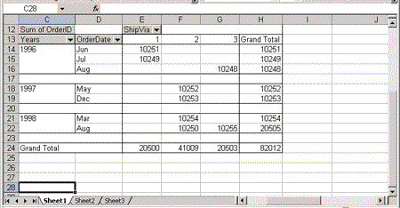
Figure 9. A PivotTable view with a blank line separating year groups

The following example specifies the values for two rows of a PivotTable view. The first field is named Discontinued and it contains integer values. The PivotItem elements specify two values for this field: 0 or 1. A blank line is inserted between the discontinued and continued items. The second PivotField element, called ProductName, specifies the inner row for the table. Since this set of values is made up of strings, the DataType element is omitted. The values for this row are Alice Mutton, Camembert Pierrot, and Carnarvon Tigers:

<PivotField>
   <Name>Discontinued</Name>
   <Orientation>Row</Orientation>
   <Position>1</Position>
   <DataType>Integer</DataType>
   <BlankLineAfterItems/>
   <PivotItem>
      <Name>0</Name>
   </PivotItem>
   <PivotItem>
      <Name>1</Name>
   </PivotItem>
</PivotField>
<PivotField>
   <Name>ProductName</Name>
   <Orientation>Row</Orientation>
   <Position>2</Position>
   <PivotItem>
      <Name>Alice Mutton</Name>
   </PivotItem>
   <PivotItem>
      <Name>Camembert Pierrot</Name>
   </PivotItem>   
   <PivotItem>
      <Name>Carnarvon Tigers</Name>
   </PivotItem>
</PivotField>

Cell Values

PivotField elements are also used to define the data in the table. For each data field, a separate PivotField element is required. The Name of the PivotField element is typically created from the aggregation being performed and the name of the underlying field (for example, "Count of Orders"). The underlying data field is specified in the ParentField element. The Orientation element must be set to "Data". The Function element specifies the aggregation being performed. Acceptable values are the following:

• Sum: Sum the data in the column
• Count: Count the number of rows even if the field is empty
• CountNums: Count of rows with data
• Avg: Average
• Max: Maximum value
• Min: Minimum value
• Product: The result of multiplying all values
• StdDev: Standard deviation
• StdDevp: Standard deviation; assumes the entire population is available rather than just a sample
• Var: Variation
• Varp: Variation; assumes the entire population is available rather than a sample

If the Function element can be omitted, by default character data is counted and numeric data is summed.

Where more than one data item is used, the Position element must also be present. The PivotField element with a Position element value of 1 is the top item in each row, the PivotField element with a Position element value of 2 is below it, and so on.

In the following example, two data fields are specified ("Sum of UnitPrice" and "Count of Items Ordered"). The Sum of UnitPrice field is displayed on top:

<PivotField>
   <Name>Sum of UnitPrice</Name> 
   <ParentField>UnitPrice</ParentField> 
   <Orientation>Data</Orientation> 
   <Position>1</Position> 
</PivotField>
<PivotField>
   <Name>Sum of ItemsOrdered</Name> 
   <ParentField>ItemsOrdered</ParentField> 
   <Orientation>Data</Orientation> 
   <Function>Count</Function>
   <Position>2</Position> 
</PivotField>

PTLineItems

The PTLineItems element holds the PTLineItem elements that define the data columns and rows in the table. Two PTLineItems are required: one specifies the rows and one specifies the columns. (The PTLineItems element for the columns must begin with an Orientation element holding the text "Column".)

A PTLineItem is required for each data PivotItem that appears in a row or a column PivotField. PTLineItems are associated with their corresponding PivotItems by position, so the first PTLineItem in the row headings corresponds to the first PivotItem element with a Position element value of 1 in the PivotField element. Each PTLineItem element contains an Item element that represents the item's position in the row or column.

The two PTLineItems elements in the following example define a set of three rows and four columns within a PivotTable view:

<PTLineItems>
   <PTLineItem>
      <Item>0</Item> 
   </PTLineItem>
   <PTLineItem>
      <Item>1</Item> 
   </PTLineItem>
   <PTLineItem>
      <Item>2</Item> 
   </PTLineItem>
</PTLineItems>
<PTLineItems>
   <Orientation>Column</Orientation
   <PTLineItem>
      <Item>0</Item> 
   </PTLineItem>
   <PTLineItem>
      <Item>1</Item> 
   </PTLineItem>
   <PTLineItem>
      <Item>2</Item> 
   </PTLineItem>
   <PTLineItem>
      <Item>3</Item> 
   </PTLineItem>
</PTLineItems>

The simplest version of a PivotTable view has just a single row with column headers, and a single data item. In this PivotTable view, the Item fields simply increment from 0 (as in the previous example). To add a totals column to your table, include a PivotItem element with an ItemType element in it that contains the string "Grand". In the following example, a grand total is added to the end of each row:

<PTLineItems>
<PTLineItem>
   <Item>0</Item> 
</PTLineItem>
<PTLineItem>
   <Item>1</Item> 
</PTLineItem>
<PTLineItem>
   <Item>2</Item> 
</PTLineItem>
<PTLineItem>
   <ItemType>Grand</ItemType>
   <Item>0</Item>
</PTLineItem>
</PTLineItems>

Other options for ItemType element specify different kinds of subtotals for a line item:

• Sum: Sum the data in the column
• Count: Count the number of rows even if the field is empty
• CountNums: Count of rows with data
• Avg: Average
• Max: Maximum value
• Min: Minimum value
• Product: The result of multiplying all values
• StdDev: Standard deviation
• StdDevp: Standard deviation; assumes the entire population is available rather than just a sample
• Var: Variation
• Varp: Variation; assumes the entire population is available rather than a sample
• Default: Sum for numeric data; Count for non-numeric data
• Blank: Inserts a blank line (a spacer)

Multiple totals can be specified by inserting multiple PTLineItems.

Where two data elements are included in each row, two PTLineItem items are required for each cell. The DataField element within the PTLineItem specifies which of the Data fields is being referred to. If the DataField is omitted, it defaults to 1.

In the following example, PTLineItems are defined for a PivotTable containing two elements in each row. The DataField element in the second PTLineItem indicates that the PTLineItem is referring to the second Data field. The DataField item is omitted for the first PTLineItem and therefore defaults to 1:

<PTLineItem>
   <Item>0</Item> 
</PTLineItem>
<PTLineItem>
   <DataField>2</DataField> 
   <Item>0</Item> 
</PTLineItem>
<PTLineItem>
   <Item>1</Item> 
</PTLineItem>
<PTLineItem>
   <DataField>2</DataField> 
   <Item>1</Item> 
</PTLineItem>

To include totals for a table that includes multiple data items, you must specify multiple total items, as in the following example:

<PTLineItem>
    <ItemType>Grand</ItemType>
    <Item>0</Item>
</PTLineItem>
<PTLineItem>
    <ItemType>Grand</ItemType>
    <DataField>2</DataField>
    <Item>0</Item>
<PTLineItem>

For multiple row or column headers, additional PTLineItems are required. As an example, assume that there are two levels of row headings: customer and shipping methods. There are three different shipping methods, so each customer entry can have three different shipping methods. The possible combinations for two customers can be expressed as follows:

Customer 1, Shipping Method 1
Customer 1, Shipping Method 2
Customer 1, Shipping Method 3
Customer 2, Shipping Method 1
Customer 2, Shipping Method 2
Customer 2, Shipping Method 3

The PTLineItem elements reflect this repeating pattern using the CountOfSameItem element to indicate that the external item is repeating. The following example demonstrates the internal row heading repeating three times for each instance of the external row heading. Both row headings begin with the first customer and shipping method (item 0). In the second entry, however, the outside row header— the customer— is repeated, as indicated by the CountOfSameItem tag, while the inside row element moves on to the second shipping method. The third PTLineItem moves to the third shipping entry in the inside row while continuing the customer in the outside row:

<PTLineItem>
   <item>0</item>   
   <item>0</item>
</PTLineItem>
<PTLineItem>
   <CountOfSameItem>1</CountOfSameItem>   
   <item>1</item>            
</PTLineItem>
<PTLineItem>
   <CountOfSameItem>1</CountOfSameItem>   
   <item>2</item>            
</PTLineItem>

For the next repetition, the document moves to the second customer in the outside row header while starting over with the first shipping method. The second PTLineItem shows the outside row repeated with the second shipping method displayed, and so on:

<PTLineItem>
   <item>1</item>   
   <item>0</item>
</PTLineItem>
<PTLineItem>
   <CountOfSameItem>1</CountOfSameItem>   
   <item>1</item>            
</PTLineItem>
<PTLineItem>
   <CountOfSameItem>1</CountOfSameItem>   
   <item>2</item>            
</PTLineItem>

PTSource

The PTSource element provides information on how the data in the PivotTable element is used. (Like the other elements associated with the PivotTable element, this element is part of the Excel namespace.) If the PTSource and PTCache elements are omitted, Excel buildsboth of them.

The key element is the first child, CacheIndex. The PTSource element ties the PivotTable element to the PivotCache that contains the data used in the PivotTable view. This example ties the PivotTable to the PivotCache element with a CacheIndex of 1:

<x:PTSource>
<x:CacheIndex>1</x:CacheIndex>
</x:PTSource>

The following elements provide information on when the data in the PivoTable view is last refreshed from the cache:

• VersionLastRefresh: The version of Excel in which the last update occurred
• RefreshName: The name of the person who last updated the PivoTable view
• RefreshDate: The date of the last update
• RefreshDateCopy: Duplicates the RefreshDate
• RefreshOnFileOpen: When present, the data is refreshed when the file is opened in Excel

Next, a ConsolidationReference element points to the data within the spreadsheet. The FileName element specifies the name of the file and the spreadsheet in that file that contains the data. The Reference element contains the actual range of the spreadsheet with the data:

<ConsolidationReference>
    <FileName>[Book2.xml]Sheet1</FileName>
    <Reference>R1C1:R26C12</Reference>
</ConsolidationReference>

Mapping XML Documents

In Microsoft Office Excel 2003, cells in a spreadsheet can be mapped to XML elements and attributes. After a mapping between a schema and an Excel spreadsheet is established, an XML data source can be bound to the spreadsheet. Excel movesdata out of the XML data source into the mapped cells for the user to view or change. When the user is finished, the spreadsheet can be saved as an XML document, and Excel moves the data out of the mapped cells into the appropriate elements or attributes.

This functionality is represented in an XML spreadsheet with the MapInfo and Binding elements. Within the MapInfo element, the Schema and Map elements contain information about the schemas being mapped and the mappings between the elements and attributes in the schema and the cells in the spreadsheet. The Binding element handles connecting the Excel spreadsheet to the XML data source.

All elements are part of the Excel2 namespace unless otherwise noted.

Mapping Information

The MapInfo element is a child of the Workbook element, appearing after the PivotCache and Name elements. The MapInfo element has two attributes, HideInactiveListBorder and SelectionNamespaces. The HideInactiveListBorder attribute, when set to true, prevents bound cells from being highlighted in the Excel user interface when the input focus isn't in one of the cells. The cells is still highlighted when the user moves the input focus to a cell in the list.

Before discussing the SelectionNamespaces attribute, it would be useful to explain the contents of the Excel2 Schema element.

Schemas

The first child of the MapInfo element is the Schema element from the Excel2 namespace. This element contains a W3C schema whose elements and attributes are to be mapped to the cells in the spreadsheet.

That SpreadsheetML uses the name "Schema" for an element that contains W3C "schemas" can make the following discussion confusing. Further confusing the issue is that the root element in a W3C schema is also named "schema". There is a difference in the names of these two elements: the Excel2 element begins with an uppercase "S" ("Schema"), and the root element of a W3C schema has a name that begins with a lowercase "s" ("schema"). Nevertheless, to prevent confusion, the SpreadsheetML Schema element in this article is referred to as the "Excel2 Schema element"; the W3C schema document is referred to as the "W3C schema" and the root element is referred to as the "W3C schema element".

In the following example, the MapInfo element has a single Excel2 Schema element which, in turn, contains a W3C schema. The contents of the W3C schema element have been omitted:

<x2:MapInfo 
      x2:HideInactiveListBorder="false"
      x2:SelectionNamespaces="xmlns:ns1='SalesOrder'">
<x2:Schema x2:ID="Schema1" x2:Namespace="SalesOrder">
<xsd:schema targetNamespace="SalesOrder">
   ...schema contents...
</xsd:schema>
</x2:Schema>

The SelectionNamespaces attribute of the Excel2 Schema element contains a list of all of the namespaces used in the W3C schema. The namespaces are specified by concatenating "xmlns" definitions that would appear in an XML document that used the schema. (The definitions are separated by a space.) If the schemas were added through in Excel, the prefixes used in these "xmlns" attributes are generated by Excel with the pattern "nsn". As an example, if two schemas with target namespaces of "Namespace1" and "Namespace2" were being mapped, the selectionNamespaces attribute would look like the following example if the schemas were added in Excel:

x2:SelectionNamespace="xmlns:ns1='Namespace1' xmlns:ns2= 'Namespace2'"

You can use any prefix that you want when you create your XML spreadsheet.

The Excel2 Schema element has three attributes:

• ID: Contains a unique ID for the W3C schema. (When Excel generates the ID value, the name is in the format "Scheman", for example, 'Schema1'.)
• Namespace: Contains the Namespace to be used with the schema. If the W3C schema inside the Excel2 Schema element has a targetNamespace, the value of this attribute must match the value in the W3C schema's targetNamespace.
• SchemaRef: Contains the ID for any Excel2 Schema element that holds a W3C schema that this schema imports.

For example, if the W3C schema "Master" uses an element defined in the W3C schema "Child," the Excel2 Schema element that contains the "Master" schema specifies a SchemaRef attribute that contains the value of the ID attribute of the Excel2 Schema element containing the "Child" schema. If a schema depends on multiple schemas, all of the IDs appear in this attribute, separated by spaces.

Frequently, one schema references elements defined in another schema. Within a W3C schema that references other schemas, the import element pulls in the other schema. The import element has an attribute called schemaLocation that points to the schema containing the referenced element. Within Excel, the schemaLocation of any import statement holds the value of the ID attribute for the Excel2 Schema element that holds the other schema.

The following example shows two schemas imported into Excel. The second schema references an element defined in the first schema. Some points to note:

The identifier for the first schema is "Schema1" as shown in the ID attribute of the Excel2 Schema element that contains the W3C schema. The identifier for the second schema is "Schema2".

The targetNamespace for the first schema is "Child"; the targetNamespace for the second schema is "Master". The Excel2 Schema element for each W3C schema has a Namespace attribute that matches the W3C schema's targetNamespace.

The second schema references an element from the first schema. To implement this, the second schema contains the import element with its schemaLocation element set to the value of ID attribute from the excel2 Schema element that holds the first schema.

Also, in order for the second schema to be able to use an element from the first schema, the Excel2 Schema element that holds the second schema has a SchemaRef attribute that points to the first schema (again, through the ID attribute of the Excel2 Schema element):

<x2:Schema x2:ID="Schema1" x2:Namespace="Child">
<xsd:schema targetNamespace="Child" 
xmlns:xsd="http://www.w3.org/2001/XMLSchema" 
xmlns="Child">
...schema details...
</xsd:schema>
</x2:Schema>
<x2:Schema x2:ID="Schema2" x2:Namespace="Master" x2:SchemaRef="Schema1">
<xsd:schema targetNamespace="Master" 
xmlns="Master" 
xmlns:c="Child" 
xmlns:xsd="http://www.w3.org/2001/XMLSchema" >
   <xsd:import namespace="Child" schemaLocation="Schema1"/>
   ...schema details...
   </xsd:schema>
</x2:Schema>

You need one Excel2 Schema element for every Schema that is used in the XML spreadsheet.

It's not necessary, however, to include all of the schemas that reference each other when you create your XML spreadsheet. Typically, there is a single schema that is the root schema for the document that you are mapping, and this schema imports all the other schemas. You need only to add this schema to your XML spreadsheet, and you can allow the schema's import statements to continue referencing the supporting schemas' files. When Excel loads your XML spreadsheet, the other schemas is loaded automatically and the necessary adjustments are made to the SchemaRef attributes and the import statements.

Keep in mind that the SpreadsheetML validation process does not validate the contents of the W3C schemas.

Mapping the Schemas

The mappings between the schema's elements or attributes and cells in the spreadsheets are held in the Map element.

Map Element

You need one Map element for each schema that has elements or attributes mapped into the spreadsheet. The attributes of the Map element are the following:

• ID: A unique identifier for the Map
• SchemaID: Holds the value of the ID attribute for the excel2 Schema element that is used by this Map.
• RootElement: The unqualified name of the root element of the schema
• Entry: Specifies a mapping between cells and elements or attributes. There is one Entry element for each mapped cell
• ShowImportExportValidationErrors: If present, this element prevents a spreadsheet from being saved if the result is not valid against the associated schema.

In the following example, an ID attribute with the value "MapSalesOrder" is defined for the Map element. The SchemaID attribute ties this Map element to the Excel2 Schema element that has "SalesOrder" in its ID attribute. The root element is called "SO":

<x2:Map 
x2:ID="MapSalesOrder" 
x2:SchemaID="SalesOrder" 
x2:RootElement="SO">

Entry Element

The Entry elements define the mappings between cells in the spreadsheet and the elements or attributes in the schema specified in the parent Map element. Excel supports two kinds of mappings between cells and schemas elements or attributes:

• Single Cell: An element or attribute is mapped to a single cell.
• Table: One or more repeating elements or attributes are mapped to the spreadsheet.

A single cell mapping ties a cell to an element (or an attribute on an element) that appears once in a document. However, often an element can appear many times in a single XML document. To support that, table mappings map repeating elements or attributes to columns in the spreadsheet.

You should think of a table a set of adjacent lists that are treated as a group. Each list occupies a column in Excel. The first row in the list can hold the name of the element or attribute mapped to the list. Subsequent rows in the column hold the values of the repeating data element or attribute. At the end of the list, you can have a cell holding some aggregate values for the list (for example, a total of the values in the list, a count of the number of items, etc.). Users can add new items to the list, effectively generating new elements or attributes in the document.

The contents of the Entry element is different depending on which mapping is being implemented.

The Entry element has the following children:

• Range: The address of the cell mapped by this entry. For single-cell mapping, the address is for the cell being mapped. For a table mapping, the address is a range. The range runs from the top left cell of the table to the last column in the table and one row down. The address is in R1C1 reference style, using absolute addressing and it includes the name of the spreadsheet. If the table consists of a single column, only the address of the topmost cell appears, with the spreadsheet name.
• FilterOn: If set to true, the list's filter is applied. This element is part of the Excel namespace.
• XPath: An XPath statement that points to the elements or attributes being mapped. For a single-cell mapping, the XPath statement specifies the element or attribute. For a table mapping, the XPath statement points to the parent element. The XPath statement must begin at the root and use the prefixes established in the SchemaRef attribute of the Excel2 Schema element.
• Field: Specifies the cell (or cells) in the spreadsheet that are being mapped. For a single-cell mapping, there is a single Field element. For a table mapping there is one Field element for each element or attribute being mapped (which may be a single Field element if only one repeating element is mapped).
• HeaderRange: Only used in table mappings. This element holds an absolute reference (in R1C1 format) to the first cell in the row of headers for a table mapping.

The Entry element also has three attributes:

• ID: Provides a unique identifier for the Entry element.
• Type: Indicates what kind of mapping takes place. The Type attribute must be set to either "single" (for a single cell mapping) or "table" (for table or list mapping).
• ShowTotals: Only for lists and tables. If an aggregation type is set in the Aggregate element (discussed in the next section) then, when this attribute is set to "true", a total row is displayed.

In the following example, the Entry element is bound to a single cell and has the ID of "1". The mapping implemented in this Entry element is for the cell F6 it links the cell to the SONumber element, which is a child of the SO element:

<x2:Entry x2:Type="single" x2:ID="1">
    <x2:Range>Sheet1!R6C6</x2:Range>
    <x:FilterOn>False</x:FilterOn>
    <x2:XPath>/phv1:SO/phv1:SONumber</x2:XPath>
</x2:Entry>

In the following example, a schema that contains an OrderLine element with two children called Product and Quantity is assumed. A table mapping is specified that associates the child elements of the OrderLine element with a range of cells beginning at D4. The elements in the schema are specified in the XPath element, which holds an XPath statement that refers to the OrderLine element (the parent of the two mapped elements). Because there are two children for the OrderLine element (Product and Quantity), two columns in the spreadsheet are needed to the hold the data. The range must also include two rows (one for headings, one for data), so the complete range is from D4 to E5 (R4C4:R5C5).

<x2:Map 
x2:ID="MapSalesOrder" 
x2:SchemaID="Schema1" 
x2:RootElement="SO">
    <x2:Entry x2:Type="table" x2:ID="24" x2:ShowTotals="false">
        <x2:Range>Sheet1!R4C4:R5C5</x2:Range>
        <x2:HeaderRange>R3C4</x2:HeaderRange>
        <x:FilterOn>True</x:FilterOn>
        <x2:XPath>/phv1:SO/phv2:Product</x2:XPath>
    </x2:Entry>
</x2:Map>

In the following example, only a single repeating attribute is mapped. A schema that contains an element called Product with an attribute called ProductID is assumed. (But, at this level, the attribute doesn't appear in the XML). The first item is put in cell A2, with the heading for the list in cell A1. The XPath element points to the element that the attribute is on:

<x2:Map x2:ID="SOMap" x2:SchemaID="Schema1" x2:RootElement="SO">
    <x2:Entry x2:Type="table" x2:ID="5" x2:ShowTotals="false">
        <x2:Range>Sheet1!R2C1</x2:Range>
        <x2:HeaderRange>R1C1</x2:HeaderRange>
        <x:FilterOn>True</x:FilterOn>
        <x2:XPath>/ns1:so/ns1:Product</x2:XPath>
    </x2:Entry>
</x2:Map>

Field Element

The Field element specifies which cells in the spreadsheet are to be mapped to the data pointed to by the XPath element. The Field element has these children:

• XSDType: The data type of the element or attribute being mapped, using the data types from the W3C Schema specification. If no data type is specified in the schema, then the value anyType is assumed.
• Cell: This is the Cell element from the spreadsheet namespace. It's used to contain formatting information for the cell.
• DataValidation: This is the DataValidation element from the Excel namespace. It holds rules to be used to check the data entered into the cell in Excel. (See the section on DataValidation for more information.)
• Aggregate: Indicates the kind of aggregation to be done in the totals row. Values are None, Sum, Count, CountNums, Var, Average, StdDev, Max, Min. The result is only displayed if the ShowTotals attribute of the Entry element is set to true.
• AutoFilterColumn: This is the AutoFilterColumn element from the Excel namespace. This controls which cells are displayed in Excel. The filter is applied only if the FilterOn element is present under the Entry element. (See the section on Filtering for more information.)
• Range: This element is used only for table mappings. This Range element is a relative address that specifies which column is to be used for each of the elements mapped from the XML document. The range is a relative address in R[1]C[1] format but, since it points only to a column, a number is required for the row. All addresses are specified from the first column in the area being used for the data. The first column is referred to as RC, the second column as RC[1], and so on.
• XPath: This element is used only for table mappings. The XPath statement is a relative path from the parent element (which is mapped in the XPath statement in the Entry element that this field element is the child of) to the child element that is to be mapped to the column specified in the Range element.

The Field element also has an ID attribute, which assigns a unique identifier to the element.

The following example shows the Field element for a single cell mapping. Only the data type is required:

<x2:Field>
    <x2:XSDType>integer</x2:XSDType>
</x2:Field>

The following example extends the previous example by adding two columns. Two Field elements are required: one for the Product element and one for the Quantity element. Within each Field element, the XPath statement specifies which element in the schema is to be used. For the first Field element, the XPath statement points to the Product element. In the second Field element, the XPath statement points to the Quantity element. For each Field element, the Range element specifies which column in the mapping's range is to be used. (The range for the table as a whole is given in the Range element under the Entry element.) For the Product element, the Range element points to the first column in the table (RC). For the Quantity element, the Range element points to the second column in the table (RC[1]).

A Count of the number of entries appears at the bottom of the list.

<x2:Field x2:ID="Product">
    <x2:Range>RC</x2:Range>
    <x2:XPath>Product</x2:XPath>
    <x2:XSDType>anyType</x2:XSDType>
    <x2:Aggregate>None</x2:Aggregate>
</x2:Field>
<x2:Field x2:ID="Quantity">
    <x2:Range>RC[1]</x2:Range>
    <x2:XPath>Quantity</x2:XPath>
    <x2:XSDType>anyType</x2:XSDType>
    <x2:Aggregate>None</x2:Aggregate>
</x2:Field>

In the following example, only a single attribute is being mapped, so only a single Field element is required. The Range element is simply RC, as is the case for the first Field element in any table mapping. The XPath statement includes the "@" character, indicating that the name after it refers to an attribute:

<x2:Field x2:ID="ProductID">
    <x2:Range>RC</x2:Range>
    <x2:XPath>@ProductID</x2:XPath>
    <x2:XSDType>string</x2:XSDType>
    <x2:Aggregate>None</x2:Aggregate>
</x2:Field>

Binding XML Data Sources

To support reading and updating an XML data source, the Binding element (a member of the Excel2 namespace) holds the connection information to find and retrieve the XML data. The primary contents of the binding element are a set of Universal Data Connection (UDC) elements, which specify the information that Excel needs to find the file.

The Binding element has two attributes:

• ID: A unique identifier assigned to the binding
• LoadMode: How the data is to be loaded. Acceptable values are "normal", "om", and "delay". When set to "normal", data is retrieved when the data source is first specified and whenever the user clicks the refresh button. In addition, the data is retrieved when the Refresh method of the Application or the XmlDataBinding objects is called. Updates are done whenever the user clicks on the update button or the Update method of the XmlDataBinding object is called. With "delay", data is not retrieved when the data source is first specified. With "om," data is only refreshed or updated when the Refresh or Update methods of the XmlDataBinding object are called.

Within the Binding element, the MapID element holds the ID of the Map element that this binding uses when working with the XML data source.

Following the MapID element are the UDC elements needed to access the data. (The UDC namespace is "http://schemas.microsoft.com/data/udc".) The DataSource element provides a container for all the UDC elements for a binding. (The DataSource's two attributes, MajorVersion and MinorVersion, specify what version of UDC the elements were written for). The Type attribute indicates which of the three kinds of data binding is being performed: SharePoint (to connect to a server that is running Windows SharePoint Services, XMLFile (for reading and writing XML files), or PartToPart (for communicating between Web Parts). Following the Type attribute, the Name attribute provides a name for the binding that is associated with the ID attribute of the Binding element. The ConnectionInfo element encloses the UDC elements specific to the binding (That is, the elements required to bind to Windows SharePoint Services, an XML file, or a Web Part). There can be multiple ConnectionInfo elements for a single data source. If there are multiple ConnectionInfo elements, the Purpose attribute distinguishes between the different connections. The values for the Purpose attribute varies depending on the kind of connection.

In the following example, a container is defined for the UDC elements that are necessary for querying an XML file:

<udc:DataSource MajorVersion="1" MinorVersion="0" >
  <udc:Type Type="XMLFile" MajorVersion="1" MinorVersion="0"/>
  <udc:Name>Binding1</udc:Name>
  <udc:ConnectionInfo Purpose="Query">

Within the ConnectionInfo element, different UDC dialects are used for different types of data access. To access a schema, the UDC XML File dialect is used. (The namespace for a UDC XML file is "http://schemas.microsoft.com/data/udc/xmlfile", and the standard prefix is "ucdxf".) The File element provides the path name to the XML file being used:

<udcxf:File >c:\SalesOrder.xml</udcxf:File>

Here's the complete set of tags to access the SalesOrder.xml file:

<x2:Binding x2:ID="Binding1" x2:LoadMode="normal">
<x2:MapID>Root_Map</x2:MapID>
<udc:DataSource MajorVersion="1" MinorVersion="0" >
<udc:Type Type="XMLFile" MajorVersion="1" MinorVersion="0"/>
<udc:Name>Binding1</udc:Name>
<udc:ConnectionInfo Purpose="Query">
<udcxf:File>c:\SalesOrder.xml</udcxf:File>
</udc:ConnectionInfo>
</udc:DataSource>
</x2:Binding>

Data Validation

Excel allows you to establish criteria for validating the data in cells in the spreadsheet. If the data entered into those cells doesn't match the criteria that you set, an error message can be displayed to the user. Optionally, you can specify a message about what data is expected. If you don't specify an error message, Excel provides a generic error message.

Specifying Tests

Data validation information is held in the DataValidation element, which is a child of the Worksheet element (appearing after any QueryTable elements and before any ConditionalFormatting elements). It is part of the Excel namespace. The child elements that control the testing are:

• Range: This element holds a string containing the range that the validation applies to, in R1C1 format.
• Type: This element specifies some constraint on the data entered into the range given in the Range element. Acceptable values are "AnyValue", "Custom", "Date", "Decimal", "List", "TextLength", "Time", and "Whole".

"Date", "Decimal", "Time", and "Whole" limit entries to those data types ("Whole" refers to whole numbers.)

"AnyValue" permits any data type (this is the default).

"TextLength" controls the amount of text entered.

"Custom" is used with the Formula element to support any kind of testing possible in Excel. The formula must return a true or false.

"List" is used with the CellRangeList element to restrict entries to items from a range in a spreadsheet.

• CellRangeList: Used with the "List" setting in the Type element, this contains a range reference in R1C1 notation, with the name of the spreadsheet, that specifies the range that contains valid values.
• Qualifier: Contains the type of test to be used to validate the cell. Acceptable values are:

"Equal", "Greater", "Less", "GreaterOrEqual", "LessOrEqual": These require the Value element.

"Between" and "NotBetween": These require the Min and Max elements. If the Min and Max elements are specified and you omit the Qualifier element, the criteria defaults to "Between".

• Value: Holds the value or the formula that is used with the qualifier to determine if the cell contains valid data. Not required for "Between" or "NotBetween".
• Min, Max: These elements are used when Type is set to "Between" or "NotBetween". They contain the value or formulas that specify the upper and lower ends of the range of valid values.
• IMEMode: Contains the status of the Input Method Editor (only relevant if East Asian language support is enabled). Valid values are "0" through "10".

Communicating with the User

Another set of elements controls the prompt displayed to the user. The prompt appears as a ScreenTip when the user selects the cell. The InputMessage specifies the message to be displayed to the user; the InputTitle specifies the title of the message tip. In the following example, the user is prompted with the date format in a ScreenTip with the title "Date Format":

<x:InputTitle>Date Format</x:InputTitle>
<x:InputMessage>Enter a date in the format yyy/mm/dd</x:InputMessage>

Another set of elements controls the error message displayed to the user if the data fails validation. The ErrorMessage element contains the actual text for the message to display. The ErrorTitle element contains the text for the caption on the message box that displays the error message. You can also use the ErrorStyle element to control the format of the message box, including the icon on the alert. Valid options for the ErrorStyle element are "Info", "Stop", and "Warn".

In the following example, a Stop message of "You must enter a valid date." is displayed if the condition's test fails. The title of the message is "Date Error":

<x:ErrorStyle>Stop</x:ErrorStyle>
<x:ErrorMessage>You must enter a valid date.</x:ErrorMessage>
<x:ErrorTitle>Date Error</x:ErrorTitle>

These four elements control options in data validation:

• InputHide: When present, prevents the input prompt from being displayed.
• ErrorHide: When present, prevents the error message from being displayed. Effectively, this turns off this data validation test.
• ComboHide: When present (and used with the List option), suppresses a drop down list box of valid values from appearing in the cell when the user selects the cell.
• UseBlank: When present (and used with the List option), prevents the cell from being tested when blank. If absent, a blank must be an acceptable entry in the list for an empty cell to be accepted.

In the following example, the cell in B10 is being checked. The validation type is set to "Whole". Only integer values (positive or negative) are therefore accepted. A minimum value of 45 and a maximum value of 200 is set as the range for the data. (The optional Qualifier element is omitted.) An input message (with a title of "Enter a value") appears as a ScreenTip when the user selects the cell, informing the user of the limits in the range. If the value entered is outside the range, a warning message (with a title of "Range Error") repeats the limits on the range:

<x:DataValidation xmlns="urn:schemas-microsoft-com:office:excel">
<x:Range>R10C2</x:Range> 
<x:Type>Whole</x:Type> 
<x:Min>45</x:Min> 
<x:Max>400</x:Max> 
<x:InputTitle>Enter a value</x:InputTitle> 
<x:InputMessage>Entry must be between 45 and 400</x:InputMessage> 
<x:ErrorStyle>Warn</x:ErrorStyle> 
<x:ErrorMessage>Value is outside the range 45 to 400.</x:ErrorMessage> 
<x:ErrorTitle>Range Error</x:ErrorTitle> 
</x:DataValidation>

Protecting and Hiding

An XML spreadsheet can be protected against changes made by the user. Protecting an XML spreadsheet allows you to protect both against changes made at the workbook level and at the worksheet level. To implement protection, you must coordinate elements and attributes at the workbook, worksheet, and cell level.

In addition to protecting your data from changes, you can also hide it from your users.

Workbook Protection

At the workbook level, you can prevent the user from making changes to the structure of the workbook (for example, by adding or removing worksheets), and from making changes to windows (for example, by freezing or unfreezing panes, splitting or unsplitting windows, and adjusting the size of windows).

The elements that control these actions are the ProtectStructure and ProtectWindows elements of the ExcelWorkbook element. (Both are members of the Excel namespace.) Setting the ProtectStructure element to true prevents structure changes; setting the ProtectWindows element to true prevents changes to the window layout.

The following example prevents changes both to the workbook structure and to the window layout:

<x:ExcelWorkbook>
  <x:ProtectStructure>True</x:ProtectStructure>
  <x:ProtectWindows>True</x:ProtectWindows>

You can set these elements independently of each other.

Worksheet Protection

To prevent changes to the worksheet, you set the Protected attribute on the Worksheet element to "1", as in this example:

<ss:Worksheet ss:Name="Sheet1" ss:Protected="1">

When a worksheet is protected, the user is not able to make changes to any cell on the worksheet unless the cell is specifically unprotected. Individual cells are unprotected by having a style applied to them that has a Protection element with its Protected attribute set to "0".

The following example defines a style called 'unprotected' and applies that style to cell C4:

<ss:Style ss:ID="unprotected">
    <ss:Protection ss:Protected="0"/>
</ss:Style>
...
<ss:Worksheet ss:Name="Sheet1" ss:Protected="1">
    <ss:Table>
        <ss:Row ss:Index="4">
            <ss:Cell ss:Index="3" ss:StyleID="unprotected"></ss:Cell>
        </ss:Row>
    </ss:Table>
</ss:Worksheet>

This strategy works well if you want to protect most of the cells in a spreadsheet and unprotect only a few (the typical case). If, however, you want to protect only a few cells, you can use the default style for the spreadsheet to unprotect most cells.

In the following example, the spreadsheet's default style specifies that cells are unprotected. Even with the Protected attribute on the worksheet set to '1', cells in the worksheet is not protected because the protection status of the default style unprotects the cells. A second style called "protected" is also defined in this example. The Protected element of this style is set to protect the cells to which the style is applied. Applying this style to any cell overrides the default style and protect the cell. The worksheet has protection turned on and cell C4 is given the "protected" style. As a result, cell C4 is protected and all other cells is unprotected:

<Style ss:ID="Default" ss:Name="Normal">
    <Protection ss:Protected="0"/>
</Style>
<ss:Style ss:ID="protected">
    <ss:Protection ss:Protected="1"/>
</ss:Style>

<ss:Worksheet ss:Name="Sheet1" ss:Protected="1">
    <ss:Table>
        <ss:Row ss:Index="4">
            <ss:Cell ss:Index="3" ss:StyleID="protected"></ss:Cell>
        </ss:Row>
    </ss:Table>
</ss:Worksheet>

When the Protection element is omitted from the default style, the default protection status for cells is controlled by the Protection attribute of the worksheet. In other words, if the default style doesn't include a Protection element, cells is protected by default in worksheets that have a Protected attribute set to 1. Cells is unprotected by default in worksheets with a Protected attribute set to 0.

Changes to the Spreadsheet

When a Worksheet element has a Protected attribute set to 1, most operations on the spreadsheet are disabled. The following table shows which elements, when added to the WorksheetOptions element, allow you to selectively enable functions for the user.

Table 5. WorksheetOption elements for protected worksheets

When these elements are absent, the corresponding ability is not permitted.

If elements are added to the WorksheetOptions element as in the following example, the user is allowed to add and delete rows and columns:

<x:WorksheetOptions>
    <x:AllowDeleteCols/>
    <x:AllowDeleteRows/>
    <x:AllowInsertCols/>
    <x:AllowInsertRows/>
</x:WorksheetOptions>

Controlling Selection

The EnableSelection element enables you to control what a user may select in a protected spreadsheet. If absent, the user can select (and copy) any cell in the spreadsheet, even if the cell is locked. When the EnableSelection element contains "UnlockedCells", the user can select only cells that have not been locked. When the element contains "NoSelection", the user is prevented from selecting any cells (that is, the user cannot copy any information in the spreadsheet). There is no option to select locked cells only. The following example illustrates how to prevent users from selecting cells:

<x:WorksheetOptions>
   <x:EnableSelection>NoSelection</x:EnableSelection>

Limitations: Scenarios, Objects, Edit Ranges, Passwords

In the WorksheetOptions element, the ProtectObjects and ProtectScenarios elements (both in the Excel namespace) can be specified. The following example illustrates a typical entry for the two elements:

<x:ProtectObjects>False</x:ProtectObjects>
<x:ProtectScenarios>False</x:ProtectScenarios>

Neither objects nor scenarios, however, can be saved in an XML spreadsheet, so preventing edits to them is unnecessary. Setting the ProtectObjects element to false does prevent the user from adding objects to a spreadsheet in Excel. Setting the ProtectScenarios element to false, on the other hand, does not prevent a user from adding a scenario to an XML spreadsheet.

Range-based information about which cells may be edited is not saved in an XML spreadsheet (that is, unprotecting cells by using the Allow Users to Edit Ranges dialog box is not supported in an XML spreadsheet).

You cannot save a workbook that is password protected as an XML spreadsheet.

Hiding

In addition to preventing changes to an XML spreadsheet, you can also hide parts of the spreadsheet. You can hide a workbook, a single worksheet within a workbook, individual columns or rows, or a cell's formula.

To hide an entire workbook, use the WindowHidden element of the ExcelWorkbook element. Users can unhide the workbook by clicking Unhide on the Window menu in Excel.

<x:ExcelWorkbook>
   <x:WindowHidden/>

To hide a single worksheet, use the Visible element in the WorksheetOptions element. Setting this element to SheetHidden hides the worksheet. Users is able to unhide the worksheet by pointing to Sheet on the Format menu in Excel and clicking Unhide. Setting the Visible element to SheetVeryHidden hides the worksheet and prevents users from unhiding it. This example hides the worksheet and prevents the user from unhiding it:

<x:WorksheetOptions>
   <x:Visible>SheetVeryHidden</x:Visible>

To hide a column or range of columns, set the Hidden attribute of the Column element to 1. To hide a range of columns, also set the Span attribute of the Column element to the number of additional columns to hide. Users is able to unhide the columns by pointing to Column on the Format menu in Excel and clicking Unhide. . This example hides column G:

<ss:Column ss:Index="7" ss:Hidden="1"/>

This example hides column G and H:

<ss:Column ss:Index="10" ss:Hidden="1" ss:Span="1"/>

To hide a row, set the Hidden attribute of the Row element to 1. Users is able to unhide the row by pointing to Row on the Format menu in Excel and clicking Unhide. This example hides row 7:

<ss:Row ss:Index="7" ss:Hidden="1"/>

Although you can't hide an individual cell, you can prevent its formula from being displayed. Do this by creating a style with a Protection element that has its HideFormula attribute set to "1". (Unlike the rest of these attributes, the HideFormula element is part of the Excel namespace. The style can then be applied to a cell. In the following example, a style called hiddenFormula is created and then used it to hide cell C4, which contains the formula "=A4"

<ss:Styles>
<ss:Style ss:ID="hiddenFormula">
<ss:Protection x:HideFormula="1" ss:Protected="0"/>
</ss:Style>
</ss:Styles>
<ss:Worksheet ss:Name="Sheet1" ss:Protected="1">
    <ss:Table>
        <ss:Row ss:Index="4">
            <ss:Cell ss:Index="3" ss:StyleID="hiddenFormula" ss:Formula="=R[-2]C"><ss:Data ss:Type="Number">0</ss:Data>
            </ss:Cell>
        </ss:Row>
    </ss:Table>
</ss:Worksheet>

Filtering Data

Autofiltering allows the user to choose to see only some of the rows in a spreadsheet by setting a filter condition on a specific column.

Turning on Filtering

The first step in using filtering is to include the FilterOn element, from the Excel namespace, in the WorksheetOptions element:

<x:WorksheetOptions>
   <x:FilterOn />
</x:WorksheetOptions>

Defining the Area

The next step in creating an autofilter is to define the filter area using a named range called "_FilterDatabase". Setting the NamedRange element's Hidden attribute to 1 prevents the area from appearing in the list of named ranges. In the following example, an autofilter is established in the area A1 to C5:

<ss:NamedRange ss:Name="_FilterDatabase" 
ss:RefersTo="=Sheet1!R1C1:R5C3"
ss:Hidden="1"/>

In addition, each cell in the range must have its NamedCell element set to the _FilterDatabase name:

<ss:Cell>
    <ss:Data ss:Type="String">Customer</ss:Data>
    <ss:NamedCell ss:Name="_FilterDatabase"/>
</ss:Cell>

Defining the Filters

The final step is to define the filters to be applied to each column. The AutoFilter element contains all the definitions in a series of AutoFilterColumn elements. (These elements are members of the Excel namespace.) The Range attribute of the AutoFilter element specifies the range to be filtered, and it must match the range defined in the _FilterDatabase named range. Setting the Hidden attribute of the NamedRange to 1 prevents the area from appearing in the list of named ranges. In the following example, an autofilter is established in the area A1 to C5:

<ss:NamedRange    ss:Name="_FilterDatabase" ss:RefersTo="=Sheet1!R1C1:R5C3" ss:Hidden="1"/>

Simple Filters

An AutoFilterColumn can be very simple. The Index element specifies which column the filter is to apply to, counting from the left, with the first column as number 1. For the filter range running from A1 to C5, this filter would apply to column C:

<x:AutoFilterColumn x:Index="3" 
x:Type="BottomPercent" x:Value="20" />

The Type attribute describes the type of filter being applied. Acceptable values are "Equals" "Top", "Bottom", "TopPercent" and "BottomPercent".

The Value attribute holds the value to be matched (for "Equals"), how many rows should be selected (for "Top" or "Bottom"), or the percentage to be selected (for "TopPercent" and "BottomPercent").

In the foregoing example, only rows with values in the bottom 20 percent of all the values in the column are to be selected.

Custom Filters

More complicated filters can be created by setting the Type attribute to "Custom". When the Type attribute is set to Custom, the Value attribute of the AutoFilterColumn is not used. Instead, a child AutoFilterCondition element is used.

The AutoFilterCondtion element's two attributes define the condition. The Operator attribute specifies the test to be done. Acceptable values are "Equals", "DoesNotEqual", "GreaterThan", "GreaterThanOrEqual", "LessThan", and "LessThanOrEqual". The Value attribute holds the value to be tested.

In the following example, the condition requires that the displayed rows not equal 14:

<x:AutoFilterColumn x:Type="Custom" x:Index="3" >
    <x:AutoFilterCondition x:Operator="DoesNotEqual" x:Value="14"/>
</x:AutoFilterColumn>

Custom filters can include up to two conditions. If two conditions are present, they must be included in either an AutoFilterAnd element or an AutoFilterOr element. When conditions appear in an AutoFilterAnd element, both must be true for the row to be displayed; with AutoFilterOr, the row is displayed if either condition is true.

In the following example, rows is displayed only if the values in the column with this filter are greater than 150 and less than 300:

<x:AutoFilterColumn x:Type="Custom">
   <x:AutoFilterAnd>
      <x:AutoFilterCondition x:Operator="GreaterThan" x:Value="150"/>
      <x:AutoFilterCondition x:Operator="LessThan" x:Value="300"/>
   </x:AutoFilterAnd>
</x:AutoFilterColumn>

Sorting

You can define a single sort area in your spreadsheet. When users select a cell in that area, they is able to re-execute the sort that you established by clicking Sort on the Data menu in Excel. A sort is defined using the Sorting element (a member of the Excel namespace). The Sorting element follows the WorksheetOptions element. The Sorting element records the options selected by the user in the Sort dialog box. Other information related to sorting (whether the sort area is to be extended to adjacent columns, For example) is not saved in the XML spreadsheet.

Within the Sorting element, Sort elements specify which columns to sort. Where the columns have headers, the Sort element contain the value of the header cell. If the columns do not have headers, the Sort element contains the name of the column in the format "Column letter" (for example, "Column A", "Column G"). If a column is to be sorted in descending order, then the Descending element must follow the column name.

If the CaseSensitive element is included, the sort distinguishes between "a" and "A" (for example, "apples" is ordered before "Apples" in the North American locale). Without the CaseSensitive element, the order of two letters that differ only in case is undefined.

The following example sorts the data by two columns, which have headers. The header in the first column is "Date Sent"; the heading in the second column is "Customer Number". The Date Sent column is sorted in descending order:

<x:Sorting>
    <x:Sort>Date Sent</x:Sort>
    <x:Descending />
    <x:Sort>Customer Number</x:Sort>
    <x:CaseSensitive />
</x:Sorting>

You can specify a custom sort order by including the Order element. Custom sort orders are based on the custom lists that you can build in Excel by using the Custom Lists tab of the Options dialog box. The Order element contains an integer that is the position in the list of custom sort orders of the sort order that you want to use. The custom lists are not saved in the XML spreadsheet.

You can also choose to sort in rows, rather than in columns. When sorting in rows you must include the LeftToRight element. When sorting in rows, you must always use the row number in the sort element. The following example sorts by Row 2:

<x:Sorting>
    <x:Sort>Row 2</x:Sort>
    <x:LeftToRight />
</x:Sorting>

Setting Up for Printing

You can set the print area to be used when Excel prints a spreadsheet. You can also provide settings for how the spreadsheet is printed, using elements in the WorksheetOptions element.

Setting the Print Area

The area to be printed is defined by a named range with the name "Print_Area". In addition, you can specify rows and columns that are to be printed on every page using a range named "Print_Titles".

In the following example, a print area from cell B6 to F10 is established. Rows 1 to 3 and columns 1 to 2 are to be printed on each page:

<ss:Names>
   <NamedRange ss:Name="Print_Area" ss:RefersTo="=Sheet1!R6C2:R10C6"/>
   <NamedRange ss:Name="Print_Titles" ss:RefersTo="=Sheet1!C1:C3,Sheet1!R1:R2"/>
</ss:Names>

Cells in these areas must have their NamedCell attribute set to the name of the range that they are part of.

Page Breaks

You can establish where new pages is start by inserting page breaks. Page breaks are defined in the PageBreaks element, which follows the WorksheetOptions element, and all of its children are members of the Excel namespace. In Excel, page breaks are marked between both columns and rows.

Within the PageBreaks element, the ColBreaks element contains all of the column breaks inside Column elements. The number inside the Column element is the number of columns between the column break and the left side of the spreadsheet (or the right side if the worksheet is configured to be viewed right to left).

In the following example, a single page break between column B and C is added:

<x:PageBreaks>
    <x:ColBreaks>
        <x:ColBreak>
            <x:Column>2<x:/Column>
        <x:/ColBreak>
    <x:/ColBreaks>
</x:PageBreaks>

The RowBreaks element holds RowBreak elements for each row break. Within the RowBreak element, a Row element contains the number of rows between the row break and the top of the spreadsheet. If the page break is within a print area, the Row break may not run the full width of the spreadsheet. Instead, ColStart and ColEnd elements mark the start and the end of the break. The ColStart and ColEnd elements specify the number of columns to the left of the break.

In the following example, a row break is established between rows 8 and 9 that runs from column B to column F, and a row break is established between column 15 and 16 that runs the full width of the spreadsheet.

<x:PageBreaks>

<x:RowBreaks>
    <x:RowBreak>
        <x:Row>8<x:/Row>
        <x:ColStart>1<x:/ColStart>
        <x:ColEnd>5<x:/ColEnd>
    <x:/RowBreak>
    <x:RowBreak>
        <x:Row>15<x:/Row>
    <x:/RowBreak>
<x:/RowBreaks>
</x:PageBreaks>

Page Break Preview

You can make Excel display a view of the page breaks in the spreadsheet. This view of page breaks allows users to adjust the position of page breaks by dragging break lines. The view is set by including the ShowPageBreakZoom element in the WorksheetOptions element. You can specify the zoom level for this display by providing a value in the PageBreakZoom element, also under the WorksheetOptions element.

These two elements (both in the Excel namespace) would cause the page break display to be shown at 200% zoom (as seen in Figure 10):

<x:WorksheetOptions>
    <x:ShowPageBreakZoom>
    <x:PageBreakZoom>200</x:PageBreakZoom>
</x:WorksheetOptions>

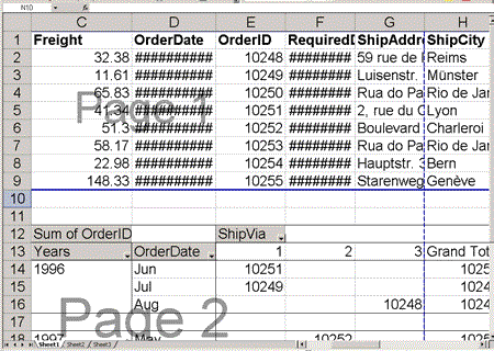
Figure 10. The page break displayed at 200% zoom

Page Layout

Most settings that relate to page layout are specified in the PageSetup element, a member of the Excel namespace.

Layout

The Layout element controls the major aspects of the how the spreadsheet appears on the page. The attributes of the Layout element include:

• Orientation: "Portrait" or "Landscape"
• CenterHorizontal: "0" for no centering or "1" to have the spreadsheet centered left to right on the page
• CenterVertical: "0" for no centering or "1" to have the spreadsheet centered top to bottom on the page
• StartPageNumber: The number to be printed on the first page

In the following example, page layout settings are configured to print the page in landscape mode, with the spreadsheet centered both horizontally and vertically on the page, and the first page numbered as 5:

<x:PageSetup>
    <x:Layout x:Orientation="Landscape"
     x:CenterHorizontal="1"
     x:CenterVertical="1"
     x:StartPageNumber="5"/>
</x:PageSetup>

Header and Footer

The attributes of the Header element control the layout of the top of the page. The Margin attribute sets the width of the top margin in inches. The Data attribute controls the text inside the header and can be separated into three areas: the area on the left, the area in the center, and the area on the right. The text for each area must appear in that order, preceded by "&L" for the material on the left, "&C" for the material in the middle, and "&R" for material on the right.

The following example shows the Data attribute for a Header element before encoding for XML. On the left side of the header "material on the left" appears; in the middle "material in the middle"; on the right "material on the right" appears:

x:Data ="&Lmaterial on the left&Cmaterial in the middle&Rmaterial on the right"

After encoding for XML, that Data attribute could be included in a Header element as in the following example:

<x:Header x:Margin="1.25"
 x:Data ="&amp;Lmaterial on the left&amp;Cmaterial in the middle&amp;Rmaterial on the right" />

The Footer element works identically to the Header element.

A set of special characters can be inserted into the Data attribute to include additional information. They are listed in the following table.

Table 6. Special characters

These special characters must be encoded for XML. As an example, to get the entry "Page 1 of 2", you would use "Page &P of &N". Encoded for XML, the string would be "Page &amp;P of &amp;N". A sample Data attribute of a header or footer in the center area, the result would look like this:

x:Data="&CPage &P of &N"   

Page Margins

The attributes of the PageMargins element are used to set the width of the margins (in inches) around the page. For the top and bottom margins, these values must be at least as large as the space set aside for the header and footer. In the following example, a margin of one and a half inches on all sides is set:

<x:PageMargins x:Bottom="1.5" x:Left="1.5" x:Right="1.5" x:Top="1.5" />

Printer Control

In addition to controlling page layout, you can specify a number of other options that control how the page is sent to the printer. The FitToPage element, if present, forces the spreadsheet to expand or contract to fill the area between the margins.

The Print element includes several elements:

• FitWidth, FitHeight: How many spreadsheet pages fit on a printed page
• LeftToRight: The direction of the print
• BlackAndWhite: Whether or not color is to be used
• DraftQuality: The quality of the print
• CommentsLayout: Where comments are to be placed. The possible values are "SheetEnd" or "InPlace". If omitted, comments are not printed.
• PrintErrors: How errors in cells are to be printed. The possible values are "NA", "Dash", and "Blank". If omitted errors are printed on the sheet.
• Scale: How much to scale up or down the size of the page, as a percentage
• PaperSizeIndex: Which size paper to use from the list of available sizes. If omitted, the default is 1.
• HorizontalResolution, VerticalResolution: The horizontal and vertical resolutions, in dots per inch
• GridLines: Whether grid lines are to be printed
• RowColHeadings: Whether row and column headings are to be printed

The following example illustrates those options. In this example, two spreadsheets are to be fit horizontally and vertically on a page. Printing is from left to right. Only black and white are to be used. The print is to be of draft quality. Comments are to be printed, but not in the cell that they are entered for. Instead, all comments are to appear following the spreadsheet. Any cells with errors is printed with the characters "NA". The spreadsheets are to be expanded 200%. The fifth paper size on the list of paper sizes is to be used. The horizontal resolution is 200 dots per inch; the vertical resolution is 100 dots per inch. Gridlines are to be printed, as are row and column headings. The result can be seen in Figure 11.

<x:Print>
    <x:FitWidth>2</x:FitWidth>
    <x:FitHeight>2</x:FitHeight>
    <x:LeftToRight/>
    <x:BlackAndWhite/>
    <x:DraftQuality/>
    <x:CommentsLayout>SheetEnd</x:CommentsLayout>
    <x:PrintErrors>NA</x:PrintErrors>
    <x:Scale>200</x:Scale>
    <x:PaperSizeIndex>5</x:PaperSizeIndex>
    <x:HorizontalResolution>200</x:HorizontalResolution>
    <x:VerticalResolution>100</x:VerticalResolution>
    <x:Gridlines/>
    <x:RowColHeadings/>
</x:Print>

Figure 11. The result of the sample printer settings

Splitting and Freezing Windows

In order to allow users to view multiple parts of a spreadsheet at the same time, Excel supports different window configurations:

• Multiple windows: The user can open as many as four windows onto the spreadsheet
• Frozen panes: The user can freeze rows along the top edge of the spreadsheet or columns on the left hand edge so that they do not scroll off the screen.
• Watch panes: The user can display a list of cells with their formulas and values.

Windows and Panes

Excel supports splitting the viewing area into multiple windows. (Up to four windows can be defined.) User can move their cursors into any of the windows and scroll within each window.

Alternatively, the viewing area can include frozen panes. With frozen panes, selected rows and columns are held on screen while the main part of the spreadsheet scrolls. Unlike a split window, a frozen pane does not scroll except to remain synchronized with the main part of the spreadsheet.

The following elements are used to configure multiple windows and frozen panes: Panes, SplitHorizontal, TopRowBottomPane, SplitVertical, LeftColumnBottomPane, FreezePanes, and FrozenNoSplit. All of these elements are children of the WorksheetOptions element and members of the Excel namespace.

Choosing Splitting or Freezing

Whether freezing or splitting is implemented is controlled by the FreezePanes and FrozenNoSplit elements. Adding these elements to an XML spreadsheet also controls what options are available to the user in switching between freezing and splitting and in returning to a single-window view.

If both elements are omitted, the window appears as split (see Figure 12). By using the Windows menu in Excel, the user can return to a single view or freeze the panes at the points where they are currently split.

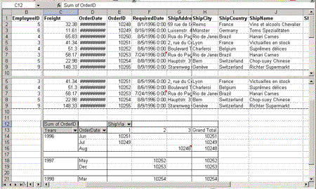
Figure 12. A split window

When the FreezePanes element is used, the frozen panes are displayed (see Figure 13). The presence or absence of the FrozenNoSplit element controls the options on the Windows menu for splitting the window at the points where it is currently frozen or returning the window to a single-pane view. These choices are summarized in the following table.

Table 7. Effect of FrozenNoSplit element

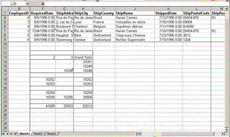
Figure 13. A window with frozen planes

The FrozenNoSplit element has no effect when used by itself.

Splitting the Window

When splitting a window, you specify two settings: the distance to the splitter bar, and which column appears first in the window on the other side of the splitter bar.

To split a window into two panes horizontally (see Figure 14), you use the SplitHorizontal and TopRowBottomPane elements. The SplitHorizontal element specifies the distance from the top of the window to the splitter bar, in points. The TopRowBottomPane specifies which row appears at the top of the lower pane. In the following example, the splitter bar is positioned 4000 points from the top of the spreadsheet's window and the top row in the lower pane is set to row 29:

<x:SplitHorizontal>3195</x:SplitHorizontal>
<x:TopRowBottomPane>29</x:TopRowBottomPane>

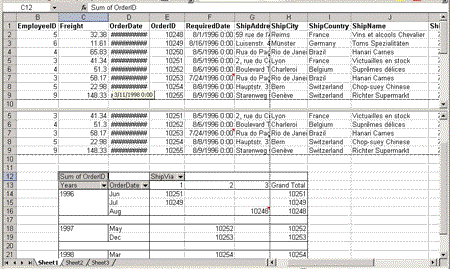
Figure 14. A window split horizontally

To split a window into two panes vertically (see Figure 15), you use the SplitVertical and LeftColumnRightPane elements. The SplitVertical element specifies the distance of the splitter bar, in points, from the left edge of the window. The LeftColumnRightPane element specifies which column appears first in the pane on the right. In the following example, the splitter bar is positioned 2000 points from the left edge and column 1 is specified as the first column in the hand pane.

<x:SplitVertical>1350</x:SplitVertical>
<x:LeftColumnRightPane>1</x:LeftColumnRightPane>

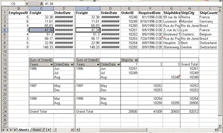
Figure 15. A window split vertically

To split a window horizontally and vertically into four panes, you use both pairs of these elements. In the following example, the horizontal splitter bar is positioned 500 points from the top edge and the vertical splitter bar is positioned 1500 points from the left edge. In the window in the lower-right pane, the cell in its upper-left corner is cell B3 (column 2, row 3):

<x:SplitHorizontal>500</x:SplitHorizontal>
<x:TopRowBottomPane>3</x:TopRowBottomPane>
<x:SplitVertical>1500</x:SplitVertical>
<x:LeftColumnRightPane>2</x:LeftColumnRightPane>

Specifying the Active Pane

Optionally, you can specify which pane has the focus when the spreadsheet is opened. You specify this by pane number, using the ActivePane element, which precedes the Panes element.

Pane numbers are based on a division of the window into four panes. The panes are numbered from 3 to 0, starting with pane 3 in the upper-left corner and counting down to pane 0 in the lower right hand corner. Pane 2 is below pane 3 and pane 1 is to the right of pane 3 (see Figure 16).

Figure 16. Four panes

If the window is not split, only pane 3 exists. If the window is split vertically, only panes 3 and 1 exist. For a horizontal split, only panes 3 and 2 exist. If the windows is split horizontally and vertically, all four panes exist.

Figure 17. No split

Figure 18. Vertical split

Figure 19. Horizontal split

The following example specifies that the ActivePane is specified as the pane in the upper-right corner. This would be valid for either a vertical or a four-way split:

<x:SplitHorizontal>500</x:SplitHorizontal>
<x:TopRowBottomPane>3</x:TopRowBottomPane>
<x:SplitVertical>1500</x:SplitVertical>
<x:LeftColumnRightPane>2</x:LeftColumnRightPane>
<x:ActivePane>1</x:ActivePane>

Specifying the Active Cell and Range

Following the settings that control the splits in the window, you can include information about each pane using Pane elements inside the Panes element.

These elements are optional and are filled in by Excel if you omit them. Each Pane element has four children:

• Number: The number that specifies which pane the element refers to
• ActiveCol: Which column contains the currently selected cell in this pane
• ActiveRow: Which row contains the currently selected cell in this pane
• RangeSelection: The last range selected in the pane

In each Pane, the ActiveCol and ActiveRow elements identify the last used cell in the pane, counting from 0. The settings of the TopRowVisible and LeftColumnVisible elements control the position of the spreadsheet in the window. As a result, the "active cell" set by the ActiveCol and ActiveRow elements may not be visible on screen if the TopRowVisible and LeftColumnVisible settings place that cell off the screen.

The RangeSelected element contains the last range selected in each pane, using R1C1 notation.

A typical use for the Pane element is to specify the current cell when the spreadsheet is opened. In the following example, the cell K7 is set as the current cell in the pane in the upper-left corner:

<x:Panes>
    <x:Pane>
        <x:Number>3</x:Number>
        <x:ActiveCol>6</x:ActiveCol>
        <x:ActiveRow>10</x:ActiveRow>
    </x:Pane>
</x:Panes>

The following example specifies a selected range:
<x:Panes>
    <x:Pane>
        <x:Number>3</x:Number>
        <x:ActiveCol>6</x:ActiveCol>
        <x:ActiveRow>10</x:ActiveRow>
        <x:RangeSelection>R4C2:R6C5</x:RangeSelection>
    </x:Pane>
</x:Panes>

Watches

The Watch window allows the user to view cells in a spreadsheet that might not all be in view simultaneously. The Excel watch window displays a selected list of cells with their current values and formulas (see Figure 20).

In an XML spreadsheet, the list of cells to be displayed is defined by the Watches element, which follows the WorksheetOptions element, and is a member of the Excel namespace. Within the Watches element, Watch elements specify the cells to be displayed in the window. Each Watch element uses a Source element that specifies the cell name (in R1C1 notation) to specify the cell to be added to the Watch window. Only a single cell can be specified in each Watch element.

In the following example, cells A1 and D5 are added to the Watch window:

<x:Watches>
    <x:Watch>
        <x:Source>R1C1</x:Source>
    </x:Watch>
    <x:Watch>
        <x:Source>R5C4</x:Source>
    </x:Watch>
</x:Watches>

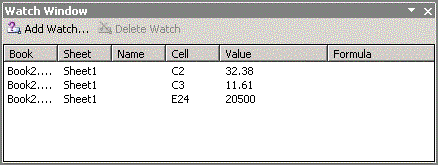
Figure 20. The Excel Watch window

Appendices

Appendix 1: Error Values

The values for the Error data type:

DIV/0!: Division by zero error

NAME?: Reference to an undefined name

NULL!: Attempt to perform an invalid calculation with the NULL value

NUM!: Invalid numeric value used

N/A: Unable to retrieve a value or value not available

REF!: Reference not valid

VALUE!: Invalid data type used

Appendix 2: AutoFormatType Values

3DEffects1

3DEffects2

Accounting1

Accounting2

Accounting3

Accounting4

Classic1

Classic2

Classic3

Colorful1

Colorful2

Colorful3

Japan1

Japan2

Japan3

Japan4

List1

List2

List3

None

PivotTableClassic

PivotTableNone

Report1

Report2

Report3

Report4

Report5

Report6

Report7

Report8

Report9

Report10

Simple

Table1

Table2

Table3

Table4

Table5

Table6

Table7

Table8

Table9

Table10

Appendix 3: SQLType Values

BigIntegerBinary

Bit

Character

Date

Decimal

Double

Float

GUID

Integer

LongVariableBinary

LongVariableCharacter

Numeric

Real

SignedBigInteger

SignedInteger

SignedSmallInteger

SignedTinyInteger

SmallInteger

Time

TimeStamp

TinyInteger

Unknown

UnsignedBigInteger

UnsignedInteger

UnsignedSmallInteger

UnsignedTinyInteger

VariableBinary

VariableCharacter

WideCharacter

WideLongVariableCharacter

WideVariableCharacter

Appendix 4: SupBook

The SupBook element contains reference information for the other spreadsheets used in formulas in the current Workbook. The SupBook element is a child of the ExcelWorkbook element and is a member of the Excel namespace. There is one SupBook element for every referenced workbook. Excel extracts the data from the referenced workbooks and store that data in the SupBook element, where it can be used in calculations without having to open the referenced workbook. Excel creates the SupBook element if it is necessary, so you don't need to add this element to your XML spreadsheet manually.

The following example illustrates a SupBook element that describes a workbook called MyOtherBook, which contains two worksheets (Sheet1 and Sheet2). The workbook is in the OtherSheets folder:

<x:SupBook>
   <x:Path>OtherSheets\MyOtherBook.xls</x:Path>
   <x:SheetName>Sheet1</x:SheetName>
   <x:SheetName>Sheet2</x:SheetName>
   <x:Xct>
 <x:Count>1</x:Count>
<x:SheetIndex>0</x:SheetIndex>
       <x:Crn>
<x:Row>3</x:Row>
<x:ColFirst>3</x:ColFirst>
           <x:ColLast>3</x:ColLast>
           <x:Number>200</x:Number>
       </x:Crn>
   </x:Xct>
   <x:Xct>
       <x:Count>0</x:Count>
       <x:SheetIndex>1</x:SheetIndex>
   </x:Xct>
</x:SupBook>

The Path element holds the path name for the referenced workbook, followed by one SheetName element for each worksheet in the workbook. The SheetName holds the name of a worksheet in the remote workbook.

Following the last SheetName is an Xct element for each worksheet. The SheetIndex element ties the Xct element to the SheetName. A "0" in the SheetIndex element indicates that this Xct element is tied to the first SheetName element in the SupBook.

The Xct element holds more detailed information about the worksheet being referenced. Within the Xct element, there must be at least one Crn element for each row that has a referenced cell in it. The Count element contains a count of the Crn elements in the Xct element.

Within the Crn element, the Row element specifies the number of the Row with a referenced cell in it. The ColFirst element specifies the number of the first column with a referenced cell. The ColLast element specifies the number of the last column with a referenced cell. As long as the referenced cells in a row have no empty cells between them, one Crn element can hold information for many referenced cells.

In the following example, the Crn element references the third row with a first and last column of 3. This Crn element, then, handles a reference to cell D3:

<x:Crn>
    <x:Row>3</x:Row>
    <x:ColFirst>3</x:ColFirst>
    <x:ColLast>3</x:ColLast>
</x:Crn>

In the following example, the Crn element references the same row as in the preceding example, but with a ColFirst element that specifies 5 and a ColLast element that specifies 10. In other words, this Crn element handles references for all cells from E3 to EJ, provided that there are no empty cells in this range:

<x:Crn>
    <x:Row>3</x:Row>
    <x:ColFirst>5</x:ColFirst>
    <x:ColLast>10</x:ColLast>
</x:Crn>

Assuming that cell D4 is empty, the two Crn elements illustrated in the next example would be required to handle references to cell D3 and D5:

<x:Crn>
    <x:Row>3</x:Row>
    <x:ColFirst>3</x:ColFirst>
    <x:ColLast>3</x:ColLast>
</x:Crn>
<x:Crn>
    <x:Row>3</x:Row>
    <x:ColFirst>5</x:ColFirst>
    <x:ColLast>5</x:ColLast>
</x:Crn>

Following the ColLast element is a series of elements for each referenced cell. This series of elements contains the data from the referenced cells. These elements must be in the same order as the cells between the ColFirst and ColLast columns. Different elements are used for different types of data: Number is used for numeric values, Text is used for string values, Boolean for Boolean values, and Error for error values.

In the following example, the Crn element is references two cells (D4 and D5). Cell D4 has a numeric value (200) and cell D5 has the text value "Hello, World":

<x:Crn>
    <x:Row>3</x:Row>
    <x:ColFirst>4</x:ColFirst>
    <x:ColLast>5</x:ColLast>
    <x:Number>200</x:Number>
    <x:Text>Hello, World</x:Text>
</x:Crn>

Appendix 5: Workbook and Worksheet Options

Not all options that are available in Excel are stored in the spreadsheet. Many of the options available in the Options dialog box in Excel do not apply to a specific spreadsheet. (An example of this kind of option is the direction that the cursor moves when the user presses the ENTER key.) However, options specific to spreadsheets can be stored in the XML spreadsheet in the ExcelWorkbook and WorksheetOptions elements. These options are listed in the following two tables.

All of these elements are optional. Many of these elements are empty elements. That is, it is the absence or presence of the element itself that configures the relevant option. Some of these elements do take values. For those elements, the default value used by Excel when the element is absent is given.

Table 8. Worksheet options

Table 9. Workbook options

See the section on managing the worksheet.

Appendix 6: PivotCache

The PivotCache element (part of the Excel namespace) contains the data to be used in a PivotTable element. The first child element inside the PivotCache is the CacheIndex element, which specifies the integer position of the cache. Following the CacheIndex is the cache information, based on the ADO Recordset model. First is a schema element (part of the XDR namespace: "uuid:BDC6E3F0-6DA3-11d1-A2A3-00AA00C14882"), which contains the description of the data that follows in the data element. The schema has an id attribute, which contains a unique identifier for the schema element.

Inside the data element, information is held in a set of elements called "row." Each field from the data source is represented by attributes with the names Col1, Col2, etc. There is one Coln attribute of the row elements for each field.

The definition of row elements is held in the Schema element using XDR syntax. Each row is described using an XDR ElementType element whose name attribute is set to "row" and whose content attribute is set to "eltOnly". Within the XDR ElementType element, a series of XDR attribute elements define the row element's attributes (each XDR attribute element has its type attribute set to "Coln" to assign names to the row element's attributes). The final element within the XDR ElementType element is the XDR extends element which has its type attribute set to "rs:rowbase".

Following the ElementType element is a series of XDR AttributeType elements (one for each Coln attribute defined in the row definition). These XDR AttributeType elements have two name attributes: one from the XDR namespace and one from rowset namespace defined by Microsoft. The s:name attribute (from the XDR namespace) is set to one of the Coln attributes. The rs:name attribute (from the rowset namespace) holds the name of the field that the Col represents.

Within the XDR AttributeType element, an XDR data type element specifies the data type of the column in its type attribute (the data types are drawn from the XDR data type specification). If string is the data type, it may be omitted, but a maxlength attribute can be used to specify the size of the string.

The following example illustrates a schema whose row element has three columns: Col1, Col2, and Col3. The Col1 attribute is a string from the CompanyName field; Col2 is the ProductId field and it is an integer; Col3 is the Quantity field and it is a float data type.

<PivotCache xmlns="urn:schemas-microsoft-com:office:excel">
    <CacheIndex>1</CacheIndex>
    <Schema s:id="RowsetSchema" 
     xmlns="uuid:BDC6E3F0-6DA3-11d1-A2A3-00AA00C14882">
        <ElementType s:name="row" s:content="eltOnly">
            <attribute s:type="Col1"/>
            <attribute s:type="Col2"/>
            <attribute s:type="Col3"/>
            <extends s:type="rs:rowbase"/>
        </ElementType>
        <AttributeType s:name="Col1" rs:name="CompanyName">
            <datatype dt:maxlength="50"/>
        </AttributeType>
        <AttributeType s:name="Col2" rs:name="ProductId">
            <datatype dt:type="int"/>
        </AttributeType>
        <AttributeType s:name="Col3" rs:name="Quantity">
            <datatype dt:type="float"/>
        </AttributeType>
    </Schema>
    <data xmlns="urn:schemas-microsoft-com:rowset">
        <row Col1="Liquid Gas Inc." Col2="213" Col3= "200.45"
         xmlns="RowsetSchema"/>
        <row Col1="Universal Widgets" Col2="157" Col3= "5"
         xmlns="RowsetSchema"/>
    </data>
</PivotCache>

Following the Schema element, the data element holds one row element for every record, with data held in the attributes defined in the preceding schema. In the example, the first record in the data element is for the company "Liquid Gas Inc" for an order of 200.45 units of product 213.

Appendix 7: Validating SpreadsheetML Documents

Validating a SpreadsheetML document does not guarantee that it loads successfully in Excel. There are many criteria for successfully loading a document that are outside the scope of XML validation. (Formulas must be defined with the correct syntax, For example.)

The reverse is also true: a document that isn't validated in the context of SpreadsheetML may well load successfully in Excel. The Schema language is far more restrictive about the order of elements than Excel is, For example. And although not having the child elements of the ExcelWorkbook element in the order specified in the SpreadsheetML schema invalidates the document as SpreadsheetML, Excel may load the document anyway.

The one certainty is that any SpreadsheetML document produced by Excel can be validated against SpreadsheetML schemas.

In addition, SpreadsheetML permits external XML tags to be embedded within a SpreadsheetML document. Many of these can be validated (for example, UDC and SOAP elements). However, there are two significant exceptions:

Smart tags are not validated. Although the SmartTagType container element is validated, the elements inside this container (which could be any of an infinite number of smart tags) are only checked to be well-formed.

W3C schemas are not validated. SpreadsheetML allows schemas representing other XML structures to be held inline inside the SpreadsheetML document.

One class of documents does not validate in the .NET environment: SpreadsheetML documents containing more than one inline schema where one schema references a definition from the other schema raises validation errors.

This following code validates a document against the SpreadsheetML schema in the .NET environment:

Function ValidateSpreadsheetMLDoc(ByVal strSchema As String, _
   ByVal strFileName As String)

Dim dom As New Xml.XmlDocument
Dim rdr As Xml.XmlTextReader
Dim xrSchema As Xml.XmlTextReader
Dim rs As New Xml.XmlUrlResolver

Try
            rdr = New Xml.XmlTextReader(strFileName)
            vr = New Xml.XmlValidatingReader(rdr)

            xrSchema = New Xml.XmlTextReader(txtSchema)

            vr.Schemas.Add("urn:schemas-microsoft-com:office:spreadsheet", xrSchema, rs)
            vr.ValidationType = Xml.ValidationType.Schema

            dom.Load(vr)

Catch excSchema As Xml.Schema.XmlSchemaException
            ValidateSpreadsheetMLDoc = False
Catch excXML As Xml.XmlException
            ValidateSpreadsheetMLDoc = False
Finally
            vr.Close()
            rdr.Close()
            xrSchema.Close()
            vr = Nothing
            rdr = Nothing
            xrSchema = Nothing
End Try

End Function

The following code validates a document against the SpreadsheetML schema in the COM environment:

Sub ValidateDoc(strSchema As String, ByVal strFileName As String)
Dim dom As New DOMDocument50
Dim bolLoadResult As Boolean
        
        Set dom = New DOMDocument50
        dom.async = False
        dom.resolveExternals = True
        dom.validateOnParse = True
        Set dom.schemas = sc
        dom.setProperty "UseInlineSchema", False

        If dom.Load(strDirectory & strFileName) = False Then
                Debug.Print dom.parseError.reason
                bolOK = False
        End If
    End Sub

The UseInlineSchema property setting prevents documents containing schemas that cross-reference each other from raising validation errors.

Appendix 8: XML Entities

Table 10. XML entities

Appendix 9: Excel Data Types

Boolean

DateTime

Number

String

Error

Appendix 10: Pivot Field Data Types

Number

Bin.Hex

Boolean

DateTime

Float

Integer

I1

I2

I8

Int

String

UI1

UI2

UI4

UI8